CS323 Compilers Notes

Outline

Introduction
Lexical Analysis
Finite Automata
Syntax Analysis
Syntax-Directed Translation
Intermediate-Code Generation
Run-Time Environments
Code Generation
Introduction to Data-Flow Analysis

Lecture 1 - Introduction

The Evolution of Programming Languages

Machine Language

1946, ENIAC
01 sequences by setting switches and cables

Assembly Language

Early 1950s
Mnemonic names for machine instructions
Macro instructions for frequently used machine instructions
Explicit manipulation of memory addresses and content
Low-level and machine dependent

High-Level Languages

2nd half of the 1950s
Fortran: for scientific computation, the 1st high-level language
Cobol: for business data processing
Lisp: for symbolic computation

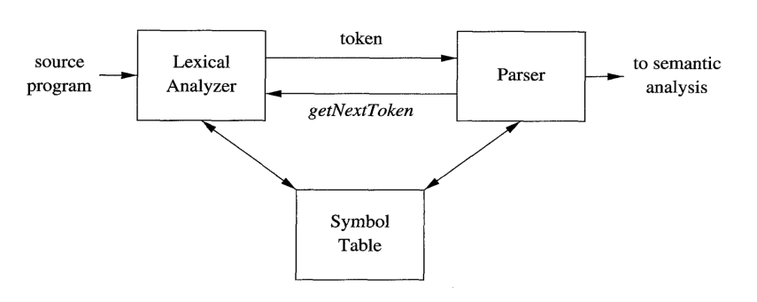
Compiler Structure

Frontend (the analysis part)	Lexical Analyzer
	Syntax Analyzer
	Semantic Analyzer
	Intermediate Code Generator
Backend (the synthesis part)	Machine Independent Code Optimizer
	Code Generator
	Machine-Dependent Code Optimizer

Frontend

Breaks up the source program into tokens
Imposes a grammatical structure on tokens
Uses the grammatical structure to create an intermediate representation
Maintains the symbol table
- variable name → storage allocated, type, scope
- procedure name → number and types of arguments, way of passing values, return type

Backend

Constructs target program from IR and the symbol table
Optimize the code

Lexical Analysis

Source code → Lexer/Tokenizer/Scanner → Tokens

Token: \

Lexemes are instances, while tokens are patterns.

Syntax Analysis

Tokens → Parser → Syntax Tree

Interior nodes: operations

Child nodes: arguments

Semantic Analysis

Syntax Tree → Syntax Analyzer → Syntax Tree

Check semantic consistency

Gather type information for type checking, type converssion, intermediate code generation.

Intermediate Code Generation

Syntax Tree → Intermediate Code Generator → IR(Three Address Code)

Assembly-like instructions
Register-like operands
At most one operator on the rhs

Machine-Independent Code Optimization

IR → Machine-Independent Code Optimizer → IR

Run faster, less memory consumption, shorter code, less power consumption…

Code Generation

IR → Code Generator → Target-Machine Code

Allocate register and memory to hold values

Compiler vs. Interpreters

Compiler

High-level language → Machine codes
Takes more time to analyze inter-statement relationships for optimization
Executable only successfully compiled

Interpreter

Directly executes each statement without compiling into machine code in advance
Takes less time to analyze the source code, simply parses each statement and executes
Continue executing until first error met

Lecture 2 - Lexical Analysis

The Role of Lexical Analyzer

Read the input characters of the source program
Group them into lexemes
Produce a sequence of tokens
Add lexemes into the symbol table when necessary

lexeme: a string of characters that is a lowest-level syntactic unit in programming languages

token: a syntactic category representing a class of lexemes. Formally, it is a pair

Token name (compulsory): an abstract symbol representing the kind of the token
Attribute value (optional): points to the symbol table

pattern: a description of the form that the lexemes of the token may take

e.g.

1	printf("CS%d",course_id);

Lexeme	`printf`	`course_id`	`"CS%d"`	`(`	…
Token	id	id	literal	left_parenthesis	…

An id token is associated with:

its lexeme
type
the declaration location(where first found)

Q: function?

Token attributes are stored in the symbol table.

Lexical error: none of the patterns for tokens match any prefix of the remaining input.

Specification of Tokens (Regex)

Alphabet: any finite set of symbols

String: (defined over an alphabet) a finite sequence of symbols drawn from an alphabet

Prefix, Proper Prefix, Suffix, Proper Suffix: n+1, n-1, n+1, n-1

Substring, Proper Substring, Subsequences: n(n+1)/2+1, n(n+1)/2-1, 2^n

String Operations

Concatenation: $x$=butter, $y$=fly, $xy$=butterfly
Exponentiation: $s^0=\epsilon, s^1=s, s^i=s^{i-1}s$

Language: any countable set$^1$ of strings over some fixed alphabet

✅The set containing only the empty string $\{\epsilon\}$ is a language, denoted $\emptyset$.

✅The set of all grammatically correct English sentences

✅The set of all syntactically well-formed C programs

$^1$A countable set is a set with the same cardinality (number of elements) as some subset of the set of natural numbers.

Operations on Languages

Union $L\bigcup M=\{s|s \text{ is in } L\text{ or }s \text{ is in }M\}$
Concatenation $LM=\{s t|s \text{ is in } L\text{ and }t \text{ is in }M\}$
Kleene closure $L^\star=\bigcup_{i=0}^{\infty}L^i$
Positive closure $L^+=\bigcup_{i=1}^{\infty}L^i$

Regex over an alphabet $\Sigma$

BASIS
- $\epsilon$ is a regex, $L(\epsilon)=\{\epsilon\}$
- If $a$ is a symbol in $\Sigma$, then $a$ is a regex, $L(a)=\{a\}$
INDUCTION: Regex $r$ and $s$ denote the languages $L(r)$ and $L(s)$
$\begin{align*} &(r)|(s) &\rightarrow &\quad L(r)\bigcup L(s)\\ &(r)(s) &\rightarrow &\quad L(r)L(s)\\ &(r)^\star &\rightarrow &\quad (L(r))^\star\\ &(r) &\rightarrow &\quad L(r) \end{align*}$

Precedence: closure $^\star$ > concatenation > union $|$

Associativity: left associative

LAW	DESCRIPTION
$r\vert s=s\vert r$	$\vert $ is commutative
$r\vert (s\vert t)=(r\vert s)\vert t$	$\vert $ is associative
$r(st)=(rs)t$	Concatenation is associative
$r(s\vert t)=rs\vert rt;\ (s\vert t)r=sr\vert tr$	Concatenation distributes over $\vert $
$r=\epsilon r=r\epsilon$	$\epsilon$ is the identity for concatenation
$r^\star=(r\vert \epsilon)^\star$	$\epsilon$ is guaranteed in a closure
$r^\star=r^{\star\star}$	$^\star$ is idempotent

e.g. Regex for C identifiers

$id\rightarrow letter_(letter_|digit)^\star$

1 2	(A\|B\|...\|Z\|a\|b\|...\|z\|_)((A\|B\|...\|Z\|a\|b\|...\|z\|_)\|(0\|1\| ...\|9))*

Regular Definitions: For notational convenience, we can give names to certain regexes and use those names in subsequent expressions.

Notational extensions

$r^+=rr^\star,\ r^\star=r^+|\epsilon$
$r?=r|\epsilon$
$[a_1a_2…a_n]=a_1|a_2|…|a_n$, $[a-e]=a|b|c|d|e$

Recognition of Tokens (Transition Diagrams)

whitespace token: ws→ (blank | tab | newline)$^+$

The lexical analyzer restarts from the next character when recognizing a whitespace token.

Transition Diagrams

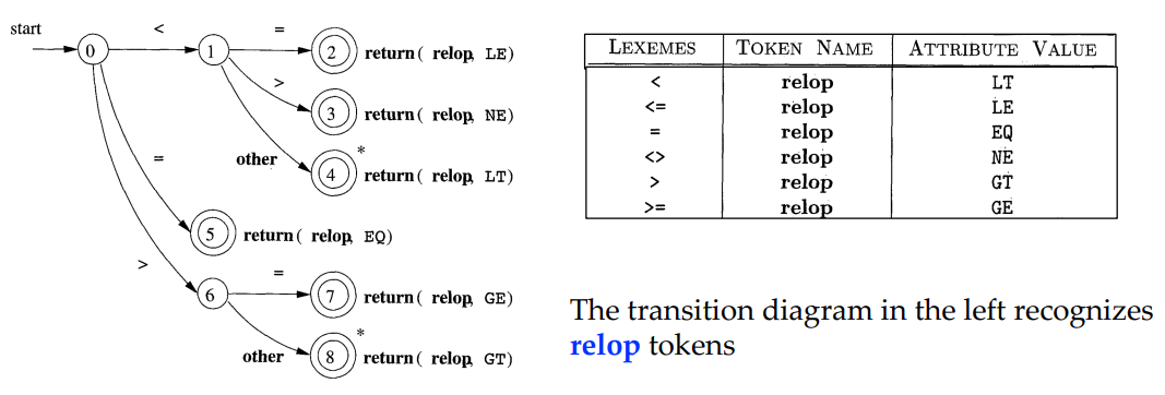
States

conditions that could occur during the process of scanning
start state: indicated by starting edge
accepting states(final): double circles

The Retract Action

Retract the forward pointer when falling into $\star$ states.

Edges: from one state to another

Handling Reserved Words

Problem: the transition diagram that searches for identifiers can also recognize reserved words

Pre-install strategy
1
return(getToken(),installID())
Multi-state transition diagrams strategy

Create a separate transition diagram with a high priority for each keyword

Building the Entire Lexical Analyzer

Try the transition diagram for each type of token sequentially
Run transition diagrams in parallel
Combining all transition diagrams into one

Lecture 3 - Finite Automata

Automata

Finite automata are graphs simply saying “yes” or “no” about each possible input string(pattern match).

Nondeterministic finite automata

A symbol can label several edges out of the same state (allowing multiple target states), and the empty string ! is a possible label.
Deterministic finite automata

For each state and for each symbol in the input alphabet, there is exactly one edge with that symbol leaving that state.

Nondeterministic Finite Automata: 5-tuple

A finite set of states $S$
A set of input symbols $\Sigma$, the input alphabet. We assume that the empty string $\epsilon$ is never a member of $\Sigma$
A transition function that gives, for each state, and for each symbol in $\Sigma\cup\{\epsilon\}$ a set of next states
A start state (or initial state) $s_0$ from $S$
A set of accepting states (or final states) $F$, a subset of $S$

Transition Table

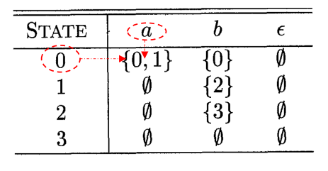
Acceptance of Input Strings

An NFA accepts an input string $x$ if and only if:

There is a path in the transition graph from the start state to one accepting state, such that the symbols along the path form $x$ ($\epsilon$ labels are ignored).

The language defined or accepted by an NFA:

The set of strings labelling some path from the start state to an accepting state.

Deterministic Finite Automata: special NFA s.t.

There are no moves on input $\epsilon$
For each state $s$ and input symbol $a$, there is exactly one edge out of $s$ labeled $a$ (i.e., exactly one target state)

From Regex to Automata

Regex→NFA→DFA

Algorithms: Thompson’s construction + subset construction

Subset construction

Each state of the constructed DFA corresponds to a set of NFA states

The algorithm simulates “in parallel” all possible moves an NFA can make on a given input string to map a set of NFA states to a DFA state.

Operations

$\epsilon$-closure($s$)

Set of NFA states reachable from NFA state s on $\epsilon$- transitions alone.

(Computed by DFS/BFS)
$\epsilon$-closure($T$)

Set of NFA states reachable from some NFA state $s$ in set $T$ on $\epsilon$-transitions alone
move($T, a$)

Set of NFA states to which there is a transition on input symbol $a$ from some state $s$ in $T$ (i.e., the target states of those states in $T$ when seeing $a$)

Dstates & Dtran

while(there is an unmarked state T in Dstates)
{
	mark T;
	for(each input symbol a)
	{
		U=epsilon-closure(move(T,a));
		if(U is not in Dstates)
		{
			add U as an unmarked state to Dstates;
		}
		Dtran[T,a]=U;
	}
}

Thompson’s Construction

The algorithm works recursively by splitting a regex into subexpressions, from which the NFA will be constructed using the following rules:

Two basis rules: handle subexpressions with no operators
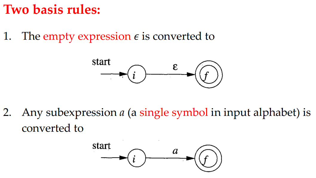
Three inductive rules: construct larger NFA’s from the smaller NFA’s for subexpressions
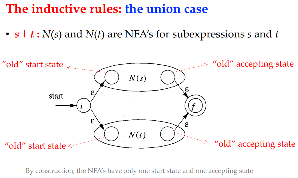
- Union
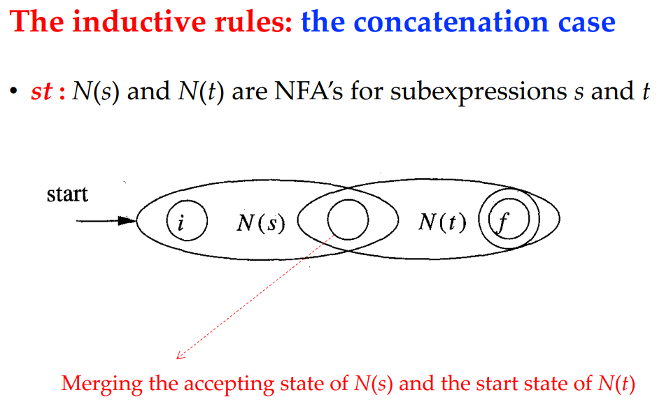
- Concatenation
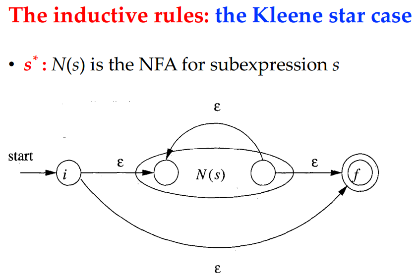
- Kleene Closure

DFA’s for Lexical Analyzers

Combining NFA’s

Why?

A single automaton to recognize lexemes matching any pattern (in the lex program)
How?

Introduce a new start state with $\epsilon$-transitions to each of the start states of the NFA’s for pattern $p_i$

The languages of big NFA is the union of the languages of small NFA’s.

Different accepting states correspond to different patterns.

DFA’s for Lexical Analyzers

Convert the NFA for all the patterns into an equivalent DFA
An accepting state of the DFA corresponds to a subset of the NFA states, in which at least one is an accepting NFA state
- If there are multiple accepting NFA states, this means that conflicts arise (the prefix of the input string matches multiple patterns)
- Solution for conflicts: pattern priority

Lecture 4 - Syntax Analysis

Introduction: Syntax and Parsers

Syntax

The syntax can be specified by context-free grammars

Grammar gives syntactic specification of a programming language, defining its structure.
For certain grammars, we can automatically construct an efficient parser
A good grammar helps translate source programs into correct object code and detect errors.

Parsers’ Roles

Obtain a string of tokens from the lexical analyzer
Verify that the string of token names can be generated by the grammar for the source language

Classification of Parsers

Universal parsers
- Some methods (e.g., Earley’s algorithm) can parse any grammar
- too inefficient to be used in practice
Top-down parsers
- Construct parse trees from the top (root) to the bottom (leaves)
Bottom-up parsers
- Construct parse trees from the bottom (leaves) to the top (root)

Context-Free Grammars

Formal definition of CFG

4 components of a CFG:

Terminals: Basic symbols token names
Nonterminals: Syntactic variables that denote sets of strings
Start symbol(nonterminal): The set of strings denoted by the start symbol is the language generated by the CFG
Productions: Specify how the terminals and nonterminals can be combined to form strings
- Format: $\text{head}\rightarrow\text{body}$
- head must be a nonterminal; body consists of zero or more terminals/nonterminals

Derivation and parse tree

Derivation: Starting with the start symbol, nonterminals are rewritten using productions until only terminals remain.

Examples.

CFG: $E\rightarrow -E\ \vert\ E+E\ \vert\ E\times E\ \vert\ (E)\ \vert\ \ \textbf{id}$

Derivation Notations

$\Rightarrow$ means “derives in one step”
$\mathop{\Rightarrow}\limits^{\star}$ means “derives in zero or more steps”
$\mathop{\Rightarrow}\limits^{+}$ means “derives in one or more steps”

Terminologies

For the start symbol $S$ of a grammar $G$, $\alpha$ is a sentential form of $G$ if $S\mathop{\Rightarrow}\limits^{\star}\alpha$.
A sentential form without nonterminals is a sentence.
The language generated by a grammar is its set of sentences.

Leftmost/Rightmost Derivations

The leftmost/rightmost nonterminal in each sentential form is always chosen to be replaced.

Parse Trees

Root node: start symbol
Leaf node: terminal symbol
Interior node: nonterminal symbol, represents the application of a production

The leaves, from left to right, constitute a sentential form of the grammar, which is called the yield/frontier of the tree.

Many-to-one: derivations→parse trees

One-to-one: leftmost/rightmost derivations→parse trees

Ambiguity

Given a grammar, if there are more than one parse tree for some sentence, it is ambiguous.

The grammar of a programming language needs to be unambiguous. Otherwise, there will be multiple ways to interpret a program

In some cases, it is convenient to use carefully chosen ambiguous grammars, together with disambiguating rules to discard undesirable parse trees

CFG vs. regexp

CFGs are more expressive than regular expressions.

$\forall L$ expressible by a regex can also be expressed by a grammar.
$\exists L$ expressible by a grammar can not be expressed by any regex.

Construct CFG from a Regex

State of NFA → nonterminal symbol
State transition on input $a$ → production $A_i\rightarrow a A_j$
State transition on input $\epsilon$ → production $A_i\rightarrow A_j$
Accepting state → $A_i\rightarrow \epsilon$
Start state → start symbol

A Context-free Language Fails Regex

$L=\{a^nb^n\vert n>0\}$

CFG: $S\rightarrow aSb\vert ab$

$L$ cannot be described by regular expressions. No DFA accepts $L$.

Proof by Contradiction

Suppose there is a DFA $D$ with $k$ states and accepts $L$.
For a string $a^{k+1}b^{k+1}$ of $L$, when processing $a^{k+1}$, $D$ must enter a state $s$ more than once.
Assume that $D$ enters state $s$ after reading the $i^\text{th}$ and $j^\text{th}$ $a$ ($i\ne j, i\le k+1,j\le k+1$).
$D$ also accepts $a^jb^j$, there exists a path labeled $b^j$ from $s$ to an accepting state.
The path labeled $a^i$ reaches $s$, then reaches an accepting state along path labeled $b^j$, so $D$ accepts $a^ib^j$. Contradiction.

Overview of Parsing Techniques

Parsing: whether the string of token names can be generated by the grammar.

Top-Down Parsing

Constructing a parse tree for the input string, starting from the root and creating the nodes of the parse tree in preorder (depth-first).

Predict: At each step of parsing, determine the production to be applied for the leftmost nonterminal.
Match: Match the terminals in the chosen production’s body with the input string.

Equivalent to finding a leftmost derivation.
At each step, the frontier of the tree is a left-sentential form.

Key decision: Which production to apply at each step?

Bottom-Up Parsing

Constructing a parse tree for an input string beginning at the leaves (terminals) and working up towards the root (start symbol of the grammar)

Shift: Move an input symbol onto the stack
Reduce: Replace a string at the stack top with a nonterminal that can produce the string (the reverse of a rewrite step in a derivation)

Equivalent to finding a rightmost derivation.
At each step, stack + remaining input is a right-sentential form.

Key decision: When to shift/reduce? Which production to apply when reducing?

Top-Down Parsing

Recursive-Descent Parsing

One procedure for each nonterminal, handling a substring of the input.

Naive procedure

void A()
{
    Choose an A-production, A → X[1-k];
    for i = 1 to k
    {
        if(X[i] is a nonterminal)
        {
            call procedure X[i]();
        }
        else if(X[i] equals the current input symbol a)
        {
            advance the input too the next symbol;
        }
        else
        {
            /* Failed to match using A-production A→X[1-k] */
        }
    }
}

Backtracking

General recursive-descent parsing may require repeated scans over the input (backtracking).

Try each possible production in some order.
When failure occurs, return, reset the input pointer and try another A-production.

Looking Ahead

Left recursion in a CFG traps the recursive-descent parser into an infinite loop.

Looking ahead, checking the next character avoids bad choices.

Computing $\text{FIRST}(X)$

$\text{FIRST}(X)$ denotes the set of beginning terminals of strings derived from $X$.

If $X$ is a terminal, $\text{FIRST}(X)=\{X\}$
If $X$ is a nonterminal and $X\rightarrow \epsilon$, then add $\epsilon$ to $\text{FIRST}(X)$.
If $X$ is a nonterminal and $X\rightarrow Y_1Y_2\cdots Y_k\ \ (k\ge1)$ is a production
- If for some $i$, $a\in \text{FIRST}(Y_i)$ and $\epsilon \in \text{FIRST}(Y_1),\cdots,\text{FIRST}(Y_{i-1})$, then add $a$ to $\text{FIRST}(X)$.
- If $\epsilon\in \text{FIRST}(Y_1),\cdots,\text{FIRST}(Y_k)$, then add $\epsilon$ to $\text{FIRST}(X)$.

Computing $\text{FIRST}(X_1X_2\cdots X_n)$

Add all non-$\epsilon$ symbols of $\text{FIRST}(X_1)$ to $\text{FIRST}(X_1X_2\cdots X_n)$.
If for some $i$, $\epsilon\in \text{FIRST}(X_1),\cdots,\text{FIRST}(X_{i-1})$, then add all non-$\epsilon$ symbols of $\text{FIRST}(X_i)$ to $\text{FIRST}(X_1X_2\cdots X_n)$.
If $\forall i,\ \epsilon\in \text{FIRST}(X_i)$, then add $\epsilon$ to $\text{FIRST}(X_1X_2\cdots X_n)$.

Computing $\text{FOLLOW}$

Whether to choose: $A\rightarrow \alpha,\ \epsilon\in\text{FIRST}(\alpha)$?

For start symbol $S$, add right endmarker $$$ to $\text{FOLLOW}(S)$.
Apply the rules below, until all $\text{FOLLOW}$ sets do not change:
- For production $A\rightarrow \alpha B\beta$, add $\text{FIRST}(\beta)/\epsilon$ to $\text{FOLLOW}(B)$
- For production $A\rightarrow \alpha B$ (or $\epsilon\in \text{FIRST}(\beta)$), then add $\text{FOLLOW}(A)$ to $\text{FOLLOW}(B)$.

By definition, $\epsilon$ will not appear in any $\text{FOLLOW}$ set.

If the next input symbol is in $\text{FIRST(body)}$, the production $\text{head}\rightarrow \text{body}$ may be a good choice.

If the next input symbol is in $\text{FOLLOW(head)}$, the production $\text{head}\rightarrow\epsilon$ may be a good choice.

LL(1) Grammars

No backtracking recursive-descent parser can be constructed for LL(1)

scanning the input from left to right.
producing a leftmost derivation (top-down parsing).
using one input symbol of lookahead each step to make parsing decision.

A grammar $G$ is LL(1) IFF for any two distinct productions $A\rightarrow \alpha\vert\beta$:

$\text{FIRST}(\alpha)\bigcap\text{FIRST}(\beta)=\emptyset$
If $\epsilon\in\text{FIRST}(\beta)$, then $\text{FIRST}(\alpha)\bigcap\text{FOLLOW}(A)=\emptyset$ and vice versa.

There is a unique choice of production at each step by looking ahead.

Parsing Table

For a nonterminal $A$ and a symbol $a$ on its input stream, determines which production the parser should choose.

The parsing table of an LL(1) parser has no entries with multiple productions.

For each production $A\rightarrow\alpha$ of grammar $G$, do the following:

For each terminal $a$ in $\text{FIRST}(\alpha)$, add $A\rightarrow\alpha$ to $M[A,a]$
If $\epsilon\in\text{FIRST}(\alpha)$, then for each terminal $b$ (including the right endmarker $) in $\text{FOLLOW}(A)$, add $A\rightarrow\alpha$ to $M[A,b]$
Set all empty entries in the table to error.

Non-Recursive Predictive Parsing

A non-recursive predictive parser can be built by explicitly maintaining a stack.

let a be the first symbol of w;
let X be the top stack symbol;
while ( X ≠ $ )
{ /* stack is not empty */
    if ( X = a ) pop the stack and let a be the next symbol of w;
    else if ( X is a terminal) error(); /* X can only match a, cannot be another terminal */
    else if ( M[X, a] is an error entry ) error();
    else if ( M[X, a] = X -> Y[1...k])
    {
        output the production X -> Y[1...k];
        pop the stack;
        push Y[k...1] onto the stack, with Y[1] on top; /* order is critical */
    }
    let X be the top stack symbol;
}

Bottom-Up Parsing

Simple LR(SLR)

Shift-Reduce Parsing

Shift zero or more input symbols onto the stack, until it is ready to reduce a string $\beta$ on top of the stack
Reduce $\beta$ to the head of the appropriate production

LR(k) Parsers

left-to-right scan of the input
construct a rightmost derivation in reverse
use $k$ input symbols of lookahead in making parsing decisions

An LR parser makes shift-reduce decisions by maintaining states to keep track of what have been seen during parsing.

LR(0) Items

An item is a production with a dot, indicating how much we have seen at a given time point in the parsing process.

The production $A\rightarrow \epsilon$ generates only $A\rightarrow \cdot$

States: sets of LR(0) items

Canonical LR(0) collection:

One collection of states, provides the basis for constructing a DFA to make parsing decisions.

Augmented Grammar

Add a new production $S^\prime\rightarrow S$ to introduce a new start symbol $S^\prime$.

$L(G)=L(G^\prime)$

Acceptance occurs IFF the parser is about to reduce by $S^\prime\rightarrow S$.

Closure of Item Sets

Grammar $G$, set of items $I$

Add every item in $I$ to $\text{CLOSURE} (I)$
If $A\rightarrow \alpha\cdot B\beta$ is in $\text{CLOSURE} (I)$ and $B\rightarrow \gamma$ is a production, then add the item $B\rightarrow\cdot \gamma$ to $\text{CLOSURE} (I)$. Repeat until no more new items can be added to $\text{CLOSURE} (I)$.

The Function GOTO

$\text{GOTO}(I,X)$ is defined to be the closure of the set of all items $[A\rightarrow \alpha X\cdot\beta]$, where $[A\rightarrow \alpha\cdot X\beta]$ is in $I$.

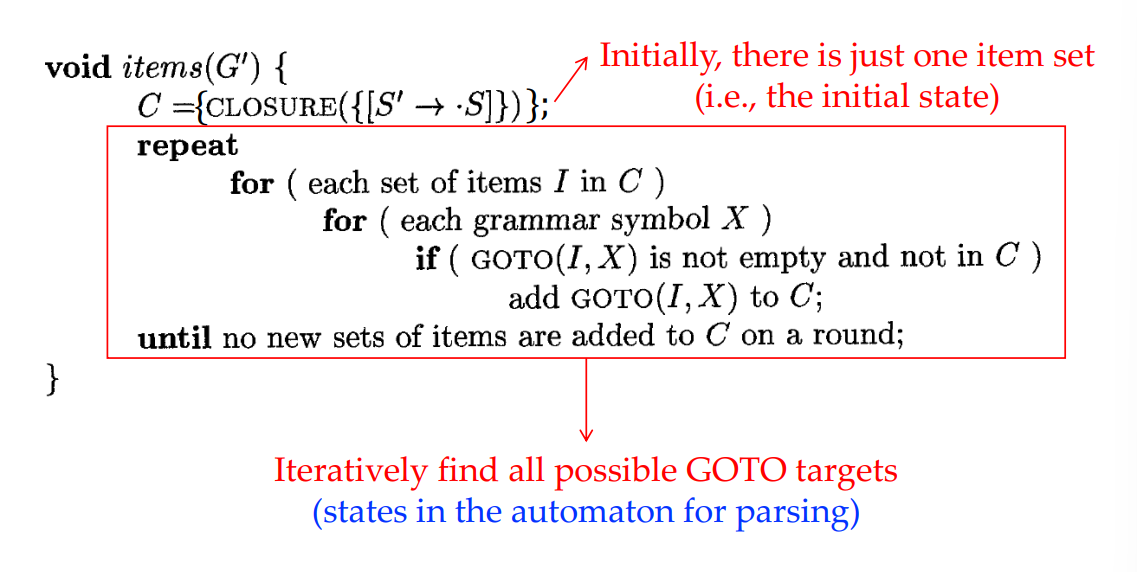
LR(0) Automaton

states: item sets in canonical LR(0) collection
transitions: GOTO
start state: $\text{CLOSURE}(\{[S’\rightarrow \cdot S]\})$

Shift when the state has a transition on the incoming symbol.

Reduce when there is no further move, push a new state into the stack corresponding to the reduced symbol.

LR Parser Structure

input, output, stack, driver program, parsing table(ACTION+GOTO)
only the parsing table differs (depending on the parsing algorithm)
stack-top state + next input terminal → next action

ACTION$[i,a]$

state $i$, terminal $a$
Shift $j$: shift input $a$ to the stack, use state $j$ to represent $a$.
Reduce $A\rightarrow \beta$: reduce stack-top $\beta$ to non-terminal $A$.
Accept: accept the input, finish parsing.
Error: syntax error detected.

LR Parser Configurations

Configuration: \

By construction, each state (except $s_0$) in an LR parser corresponds to a set of items and a grammar symbol (the symbol that leads to the state transition)

Suppose $X_i$ is the grammar symbol for state $s_i$, then $X_0X_1\cdots X_ma_ia_{i+1}\cdots a_n$ is a right-sentential form (assume no errors).

ACTION$[s_m,a_i]$

Shift $s$: $(s_0s_1\cdots s_ms,a_{i+1}\cdots a_n$)$
Reduce $A\rightarrow \beta$: $(s_0s_1\cdots s_{m-r}s,a_ia_{i+1}\cdots a_n$)$, where $r$ is the length of $\beta$, and $s=\text{GOTO}(s_{m-r},A)$

Constructing SLR-Parsing Tables

Construct canonical LR(0) collection $\{I_0,\cdots,I_n\}$ for the augmented grammar $G^\prime$.
State $i$ is constructed from $I_i$. ACTION can be determined as follows:
The GOTO transitions for state $i$ are constructed for all nonterminals $A$ using the rule: If $\text{GOTO}(I_i,A)=I_j$, then $\text{GOTO}(i,A)=j$.
All entries not defined in steps 2 and 3 are set to “error”
Initial state is the one constructed from the item set containing $[S^\prime\rightarrow\cdot S]$

If there is no conflict (i.e., multiple actions for a table entry), the grammar is SLR(1).

Weakness

Stack-top reduction: $\beta\alpha\Rightarrow\beta A$ when $a\in\text{FOLLOW}(A)$, but $a\not\in\text{FOLLOW}(\beta A)$ .

Canonical LR(CLR)

LR(1) Item: $[A\rightarrow \alpha\cdot\beta,a]$

$A\rightarrow \alpha\beta$ is a production, $a$ is a terminal or $$$.
1: length of the lookahead
The lookahead symbol only works if $\beta=\epsilon$.

$[A\rightarrow\alpha\cdot,a]$ calls for a reduction by $A\rightarrow\alpha$ only if the next input symbol is $a$.

When calculating CLOSURE, generate a new item $[B\rightarrow \cdot\gamma,b]$ from $[A\rightarrow\alpha\cdot B\beta,a]$ if $b\in\text{FIRST}(\beta a)$.

\<$\cdots\alpha\gamma,b\cdots$> → \<$\cdots\alpha B,b\cdots$> → \<$\cdots\alpha Bb,\cdots$>

$\beta=\epsilon, b=a ;\beta\not= \epsilon, b\in \text{FIRST}(\beta)\equiv b\in\text{FIRST}(\beta a)$

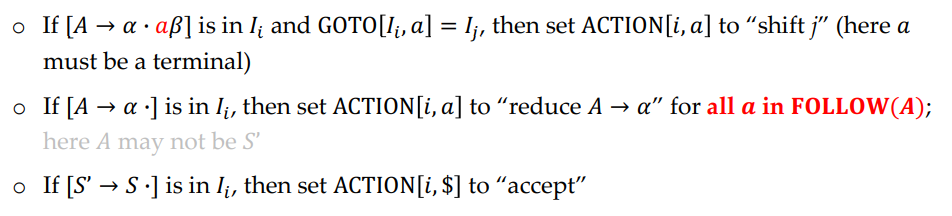
Look-ahead LR (LALR)

Merge sets of LR(1) items with the same core.

The core of an LR(1) item set is the set of the first components, a set of LR(0) items.

Merging states may cause reduce/reduce conflicts:

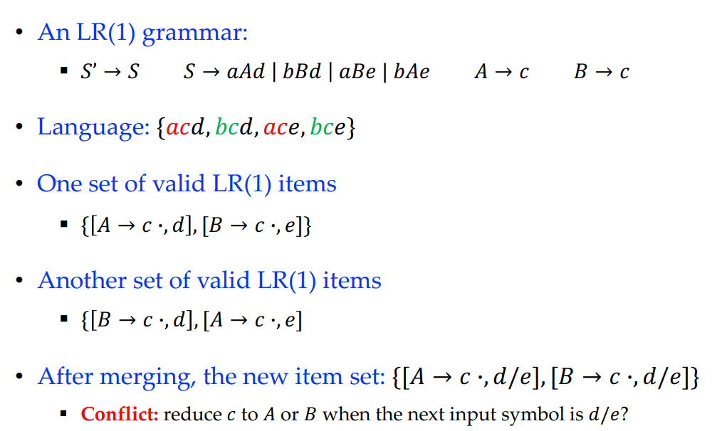
Merging states in LR(1) parsing table; If there is no reduce-reduce conflict, the grammar is LALR(1), otherwise not LALR(1).

Comparisons Among LR Parsers

Languages/Grammars supported:$\text{CLR>LALR>SLR}$

number of states in the parsing table: $\text{CLR>LALR=SLR}$

Driver programs: $\text{CLR=LALR=SLR}$

Lecture 5 - Syntax-Directed Translation

Syntax-Directed Definitions

Syntax-Directed Definitions: attributes + semantic rules

Synthesized Attributes: value at a parse-tree node $N$ is only determined from attribute values at the children of $N$ and at $N$ itself

can be evaluated during bottom-up traversal of a parse tree

Inherited attributes have their value at a parse-tree node determined from attribute values at the node itself, its parent, and its siblings in the parse tree

Non-terminals in a parse tree may not correspond to proper language constructs

Evaluation Orders for SDD’s

Dependency: $N.a = f(\{M_i.a_i\})$

Dependency Graph: defines partial relations(order of computation) between attributes

vertex: attribute instance
directed edge $a_1\rightarrow a_2$: $a_1$ is needed to compute $a_2$
cycle: cyclic dependency, not computable

Then compute the attributes in topo-sort order.

Hard to tell if an arbitrary SDD is computable (parse trees contain no cycles).

S-Attributed SDD

Every attribute is synthesized, always computable.

Edges are always from child to parent, any bottom-up order is valid, e.g., postorder traversal during bottom-up parsing.

L-Attributed SDD

Every production $A\rightarrow X_1\dots X_n$, for each $j=1\dots n$, each inherited attribute of $X_j$ only depends on:

the attributes of $X_1,\dots,X_{j-1}$
the inherited attributes of $A$

Or each attribute is synthesized, therefore S-Attributed SDD $\subseteq$ L-Attributed SDD.

Edges are always from left to right, or from parent to child, computable.

evaluate inherited attributes from parent node
evaluate child nodes from left to right
evaluate synthesized attributes from child nodes.

Syntax-Directed Translation Schemes

CFG with semantic actions embedded within production bodies

Differ from the semantic rules in SDD’s
Semantic actions can appear anywhere within a production body

$B\rightarrow X\{a\} Y$

If terminal $X$ is recognized, or all the terminals derived from nonterminal $X$ is recognized, action $a$ is done.

bottom-up: perform $a$ as $X$ appears on the top of the parsing stack
top-down: perform $a$ before attempting to expand $Y$ (if $Y$ is a nonterminal) or check for $Y$ on the input (if $Y$ is a terminal)

SDT’s Implementable During Parsing

marker nonterminals $M\rightarrow \epsilon$ to replace embedded actions
grammar parse-able, then SDT can be implemented during parsing

Lecture 6 - Intermediate-Code Generation

Front-end: Parser, Static Checker, Intermediate Code Generator

Back-end: Code Generator

Intermediate Representation

$M$ languages, $N$ machines, with intermediate representations, $M+N$ compilers.

High-level IR like syntax trees are close to the source language

machine-independent tasks

Low-level IR are close to the target machines

machine-dependent tasks

On DAG, subexp appearing multiple times → subtree with multiple parents(node reuse)

Three-Address Code

$\text{x} = \text{y op z}$

Only one operator on the rhs.

Operands(addresses) can be:

Names
Constants
Temporary names

Instructions

Assignment

$\text{x} = \text{y op z}$

$\text{x} = \text{op y}$
Copy

$\text{x = y}$
Unconditional jump

$\text{goto L}$
Conditional jump

$\text{if goto L}$
Procedure calls/returns

$\text{param x}_{1\dots n}$

procedure call: $\text{call p, n}$

function call: $\text{y = call p, n}$

$\text{return y}$
Indexed copy

$\text{x = y[i]}$

$\text{x[i] = y}$
Address and pointer assignment

$\text{x = \&y}$ (x.rval ← y.lval)

$\text{x = *y}$ (x.rval ← content stored at location indicated by y.rval)

$\text{*x = y}$ (content store at location indicated by x.rval ← y.rval)

Quadruples

$\text{op}\quad \text{arg}_1\quad \text{arg}_2\quad \text{result}$

Simple, straight forward.

Temporary names in result field are space-consuming(symbol table entries).

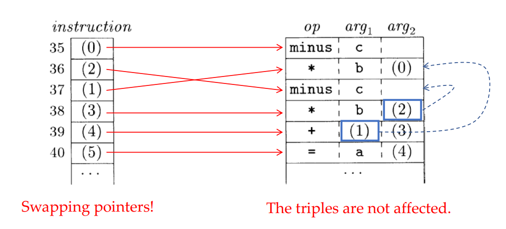
Triples

$\text{op}\quad \text{arg}_1\quad \text{arg}_2$

Refer to the results by positions, without generating temporary names.

Compiling optimization may swap instructions, leading to wrong results in triples.

Indirect Triples

Consist of a list of pointers to triples.

An optimization can move an instruction by reordering the instruction list.

Static Single-Assignment Form

Each name receives a single assignment

combine definitions in different branches using $\phi$-function

if(flag)
    x[1] = -1;
else
    x[2] = 1;
x[3] = phi(x[1],x[2]);
y = x[3] * a;

Type and Declarations

Types and Type Checking

Type info usages

Find faults
Determine memory needed at runtime
Calculate addresses of array elements
Type conversions
Choose arithmetic operator

Type checking: types of operands match the type expectation.

Type Expressions

basic type: boolean, char, integer, float, void…
type name: name of a class
type constructor
- array(number, type expression)
- record
- function(type, type)→ return type
Name Equivalence

names in type expressions are not replaced by the exact type expressions they define
Structural Equivalence

replace the names by the type expressions and recursively check the substituted trees

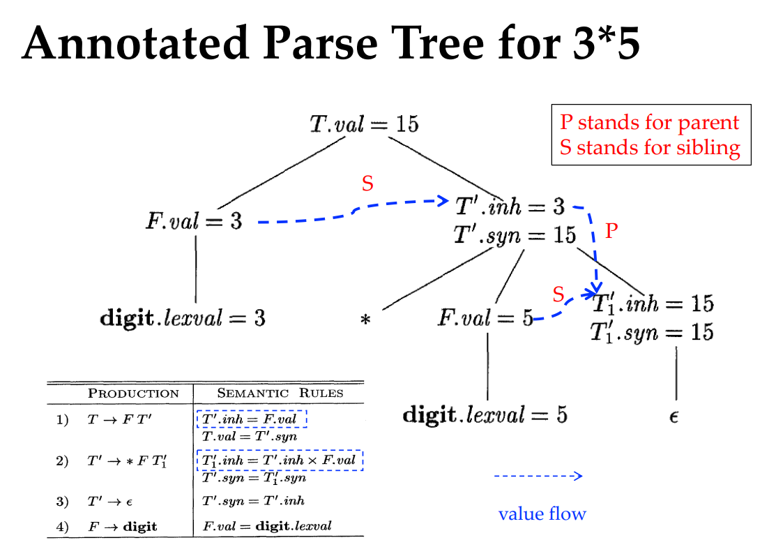
Translation of Expressions

SDD for Expression Translation

S
| id = E;
{
    S.code = E.code ||
        gen(top.get(id.lexeme) '=' E.addr);
}
E
| E1 + E2
{
    E.addr = new Temp();
    E.code = E1.code || E2.code || 
        gen(E.addr '=' E1.addr '+' E2.addr);
}
| - E1
{
    E.addr = new Temp();
    E.code = E1.code || E2.code || 
        gen(E.addr '=' 'minus' E1.addr);
}
| (E1)
{
    E.addr = E1.addr;
    E.code = E1.code;
}
| id
{
    E.addr = top.get(id.lexeme);
    E.code = '';
}

Generate instructions when seeing operations, then concatenate instructions

For id, check the symbol table and save its address
Use temporary name to hold intermediate values

Problem

code attributes may be too long. Redundant parts waste memory!

Incremental Translation Scheme

S
| id = E;
{
    gen(top.get(id.lexeme) '=' E.addr);
}
E
| E1 + E2
{
    E.addr = new Temp();
    gen(E.addr '=' E1.addr '+' E2.addr);
}
| - E1
{
    E.addr = new Temp();
    gen(E.addr '=' 'minus' E1.addr);
}
| (E1)
{
    E.addr = E1.addr;
}
| id
{
    E.addr = top.get(id.lexeme);
}

gen appends the new 3-addr instruction to the sequence of instructions.

This postfix SDT implemented in bottom-up parsing(semantic actions are executed upon reduction) guarantees that subexpressions are handled first.

Control Flow

Short Circuit Behavior

if ( x < y || x > z && x != w )
    x = 0;
/*
    if x < y goto L2
    ifFalse x > z goto L1
    ifFalse x != w goto L1
L2: x = 0
L1: 
*/

Flow-of-Control Statements

Grammar

$S\rightarrow \textbf{if} (B)\ S_1$
$S\rightarrow \textbf{if} (B)\ S_1\ \textbf{else}\ S_2$
$S\rightarrow \textbf{while} (B)\ S_1$

Inherited attributes

$B.true$: the label to which control flows if $B$ is true.
$B.false$: the label to which control flows if $B$ is false.
$S.next$: the label for the instruction immediately after the code for $S$.

1
2
3

B.code  ->	B.true/false
B.true:		S1.code
B.false:	...

if-else

B.code  ->	B.true/false
B.true:		S1.code
			goto S.next
B.false: 	S2.code
S.next:		...

while

begin:
B.code  ->	B.true/false
B.true:		S1.code
			goto begin
B.false: 	...

Three-Address Code for Booleans

B
| E1 rel E2
{
    E.code = E1.code || E2.code
        || gen('if' E1.addr rel.op E2.addr 'goto' B.true)
        || gen('goto' B.false);
}
| true
{
    B.code = gen('goto' B.true);
}
| false
{
    B.code = gen('goto' B.false);
}

B
| B1 || B2
{
    B1.true = B.true;
    B1.false = newlabel();
    B2.true = B.true;
    B2.false = B.false;
    B.code = B1.code || label(B1.false) || B2.code
}
| B1 && B2
{
    B1.true = newlabel();
    B1.false = B.false;
    B2.true = B.true;
    B2.false = B.false;
    B.code = B1.code || label(B1.false) || B2.code
}
| !B1
{
    B1.true = B.false;
    B1.false = B.true;
    B.code = B1.code;
}

Lecture 7 - Run-Time Environments

Run-Time Environment

Source-language abstractions

Names, scopes, data types, operators, procedures, parameters, flow-of-control constructs…

Run-time Environment

Layout and allocation of storage locations for data in the source program
Mechanisms to access variables
Linkages between procedures, the mechanisms for passing parameters

Storage Organization

Static:

Storage-allocation decision can be made by looking only the program text.

Global constants, global variables

Dynamic:

Storage-allocation decision can be made only while the program is running

Stack

Lifetime same as that of the called procedure
Heap

Hold data that may outlive the call to the procedure that created it

Manual memory deallocation

Automatic memory deallocation(GC)

Stack Space Allocation

Procedure calls (activation of procedures): FI(called) LO(return)

Activation tree

node: corresponds to an activation (children nodes are ordered)
root: activation of main() procedure
pre-order traversal: sequence of procedure calls
post-order traversal: sequence of returns

Activation Record

Procedure calls and returns maintained by a run-time stack: call stack(control stack)
Each live activation has an activation record (stack frame) on the control stack

Calling/Return Sequences

Calling sequences

allocating activation records on the stack
entering information into its fields

Return sequences

restoring the machine state so that the caller can continue execution

Divided between caller and callee. Put as much code as possible into the callee.

Data perspective: pass arguments and return values.

Control perspective: transfer the control between the caller and the callee.

Component	Descriptions
Actual parameters	Actual parameters used by the caller
Returned values	Values to be returned to the caller
Control link	Point to the activation record of the caller
Access link
Saved machine status	Information about the state of the machine before the call, including the return address and the contents of the registers used by the caller
Local data	Store the value of local variables
Temporaries	Temporary values such as those arising from the evaluation of expressions

Values passed between caller and callee are put at the beginning of the callee’s activation record (next to the caller’s record)

Fixed-length items (control link, access link, saved machine status) are in the middle

Items whose size may not be known early enough are placed at the end

stack top pointer sp points to the end of the fixed length fields

Steps of a calling-return sequence

The caller evaluates the actual parameters
The caller stores return address and sp into the callee’s activation record
The caller increases sp accordingly
The callee saves the register values and other status info
The callee initializes its local data and begins execution
Callee execution
The callee places the return value next to the actual parameters fields in its activation record
Using information in the machine-status field, the callee restores sp and other registers
Go to the return address set by the caller

Heap Management

The Memory Manager

Heap: data that lives indefinitely

Memory manager allocates and deallocates space within the heap

Allocation: Provide contiguous heap memory

use free space in heap
extend the heap by getting consecutive virtual memory

Deallocation: Return deallocated space to the pool of free space for reuse

memory managers do not return memory to the OS

Desirable Properties

Space efficiency
Program efficiency
Low overhead

Leveraging Program Locality

Use memory hierarchy to minimize the average memory-access time

Temporal locality
Spatial locality

Reducing Fragmentation

Fragmentation

Best-fit algorithm

improve space utilization, but slow

First-fit algorithm

faster and improves spatial locality, but fragmentation

The Doug Lea’s Strategy

Lecture 8 - Code Generation

Target Language

Three-address machine: load / store / computation / jump / conditional jump

Addressing modes

Variable name x

x‘s l-value
a(r)

a‘s l-value + value in r

a is a variable, r is a register
const(r)

const + value in r

Indirect addressing mode
*const(r)

Two indirect addressing mode
*r

Two indirect addressing mode
#const

Immediate constant addressing mode

Addresses in the Target Code

Static Allocation

Size and layout of the activation records determined by the symbol table.

Store the return address in the beginning of the callee’s activation record in the stack area
Jump to codeArea, the address of the 1st instruction of the callee in the code area
Transfer control to the address saved at the beginning of the callee’s activation record

ST callee.staticArea, #here + offset
BR callee.codeArea
...
BR *callee.staticArea

Stack Allocation

Use relative addresses for storage in activation records.

Maintain a sp register pointing to the beginning of the stack-top activation record

ADD SP, SP, #caller.recordSize
ST *SP, #here + const
BR callee.codeArea
...
BR *0(SP)
SUB SP, SP, #caller.recordSize

Basic Blocks and Flow Graph

Basic block: no halting/branching in the middle

Flow graph: basic blocks as nodes, block-following relations as edges

Partitioning Three-Address Instructions into Basic Blocks

Finding leader instructions:

The 1st instruction of the entire intermediate code
Target of any jump instruction
Instructions immediately following jump instructions

basic block: [leader instructions, min{next leader instructions, EOF})

Loops

A loop $L$ is a set of nodes in the flow graph
$L$ contains a node $e$ called the loop entry (循环入口)
No node in $L$ except $e$ has a predecessor outside $L$.
Every node in $L$ has a nonempty path, completely within $L$, to $e$

Optimization of Basic Blocks

The DAG (directed acyclic graph) of a basic block enables several code-improving transformations:

Eliminate local common subexpressions
Eliminate dead code
Reorder operands of instructions by algebraic laws

Local Common Subexpression

same operator, same children nodes in the same order, create only one node.

Dead Code Elimination

Delete any root (node without ancestors) that has no live variables attached.

Repeatedly applying the transformation until convergence.

Use of Algebraic Identities

Eliminate computations: $x\times 1 = x$
Reduction in strength: $x / 2 = x * 0.5$
Constant folding: $2 * 3.14 = 6.28$

Simple Code Generator

Three-address code→Machine instructions

Use registers wisely to avoid unnecessary load and store instructions.

Principal uses of registers

operands
temporaries
global values
run-time storage management (rsp)

Code Generation Algorithm

Generate load only when necessary, avoid overwriting register in use.

Register descriptor

Address descriptor

variable → locations storing its value (register, memory address, stack location)

getReg(I) Usages

Select registers for each memory location of 3-address instruction $I$.

$\text{x = y + z}$
1. Invoke getReg(I) to select registers $\text{R}_\text{x}, \text{R}_\text{y},\text{R}_\text{z}$.
2. If $\text{y}$ is not in $\text{R}_\text{y}$, according to the register descriptor, generate $\text{LD \ R}_\text{y},\ \text y^\prime$, where $\text y^\prime$ is the memory location for $\text y$ according to the address descriptor.
3. Generate $\text{ADD \ R}_\text x,\ \text R_\text y,\ \text R_\text z$
$\text{x = y}$
1. getReg(I) selects the same register for $\text x$ and $\text y$.
2. If $\text{y}$ is not in $\text{R}_\text{y}$, generate $\text{LD \ R}_\text{y},\ \text y^\prime$.
Ending a basic block
1. For temp variables, release the associated registers
2. If a variable is live (not 100% dead) on block exit, generate $\text{ST x},\ \text R_\text x$ for $\text x$ whose value in the register is newer than that in memory.

Updating descriptors

Values in registers are no older than those in memory.

$\text{LD \ R},\ \text x$
1. Set the register descriptor for $\text R$ to $\text x$
2. Add $\text R$ to address descriptor for $\text x$
3. Remove $\text R$ from address descriptor of other variables
$\text{ST \ x},\ \text R$
1. Add memory location of $\text x$ to its address descriptor
$\text{ADD \ R}_\text x,\ \text R_\text y,\ \text R_\text z$
1. Set the register descriptor for $\text R_\text x$ to $\text x$
2. Set the address descriptor for $\text x$ to only $\text R_\text x$
3. Remove $\text R_\text x$ from address descriptor of other variables
$\text x = \text y$
1. Use rule 1 if $\text{LD \ R}_\text y,\ \text y$ is generated
2. Remove $\text x$ from the register descriptor of $\text R_\text x$
3. Add $\text x$ to the register descriptor of $\text R_\text y$
4. Set the address descriptor for $\text x$ to only $\text R_\text y$

Select registers

Pick registers for operands and result for each three-address instruction while avoiding load and store as possible.

What if there’s no register available when attempting to allocate one?

Example: $\text x = \text y + \text z$, allocating a register for $\text y$

Check if the victim $\text R_\text v$ is safe to update
- There exists somewhere else storing latest value of $\text v$ besides $\text R_\text v$
- $\text v$ is $\text x$ (lhs) and $\text x$ is not the other operand $\text z$
- $\text v$ is dead after this instruction
If there is no safe registers, generate $\text{ST\ v, \ R}$ to store $\text v$ into its memory location (spill).

If $\text R$ holds multiple variables, repeat the process for each such variable $\text v$.

Pick the register requiring the smallest number of ST instructions.

Lecture 9 - Introduction to Data-Flow Analysis

The Data-Flow Abstraction

Data-flow analysis: Derive information about the flow of data along program execution paths.

identify common subexpressions
eliminate dead code

Program point: points before and after each statement.

Execution path: sequence of points (within block / across block).

Program execution can be viewed as a series of transformations of the program state (the values of all variables, etc.)

Input State→Statements→Output State

Data-flow analysis : all the possible program states → a finite set of facts

In general, there is an infinite number of possible paths, and no analysis is necessarily a perfect representation of the state.

Reaching definitions

The data-flow value at program point is the set of var‘s definitions that can reach this point.

Constant folding

The data-flow value for var at program point is (not) a constant.

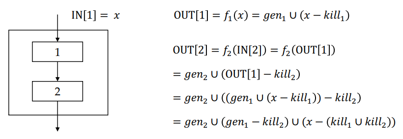
The Data-Flow Analysis Schema

Constraints based on the semantics of the statements (transfer functions)

Transfer function: the relationship between the data-flow values before and after each statement.

Forward-flow problem: information propagate forward along execution paths, $\text{OUT}[s]=f_s(\text{IN}[s])$.
Constraints based on the flow of control
1. Intra-block: $\text{IN}[s_{i+1}]=\text{OUT}[s_i]$
2. Inter-block: $\text{IN}[B]=\bigcup\limits_{P\text{ a predecessor of B}}\text{OUT}[P]$ (forward-flow)

Precise: code improvement
Constraints: correct program semantics

Classic Data-Flow Problem

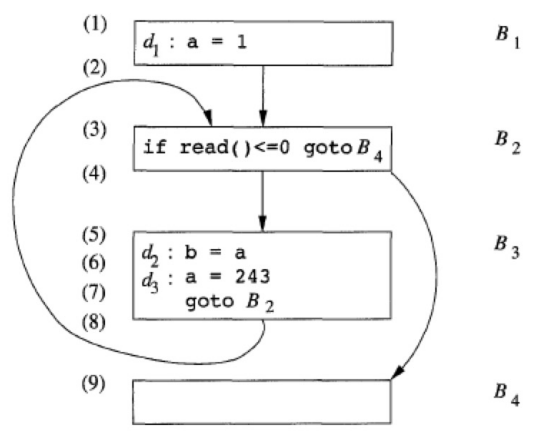
Reaching Definitions

A definition $d$ of some variable $x$ reaches a point $p$ if there is a path from the program point after $d$ to $p$, such that $d$ is not “killed” along that path.

If $d$ reaches the point $p$, then $d$ might be the last definition of $x$.

Inaccuracies are allowed, but FALSE POSITIVE(reachable definitions killed) is not acceptable.

Transfer Equations

For a statement d: u = v + w,

Generate a definition $d$ of variable $u$ and kill all other definitions of $u$.

$f_d(x) = \text{gen}_d\cup (x-\text{kill}_d)$

For a block $B$ with $n$ statements,

$\begin{align*} f_B(x) &= \text{gen}_B\cup (x-\text{kill}_B)\\ \text{gen}_B &= \bigcup\limits_{i=1}^n(\text{gen}_i-\sum\limits_{j=i+1}^n\text{kill}_j)\\ \text{kill}_B &= \bigcup\limits_{i=1}^n \text{kill}_i \end{align*}$

The kill set is the union of all the definitions killed by the individual statements.

The gen set contains all the definitions inside the block that are downward exposed (visible immediately after the block).

Control-Flow Equations

For the ENTRY block: $\text{OUT}[\text{ENTRY}] = \emptyset$

For any other basic block $B$:

$\begin{align*} \text{OUT}[B] &= \text{gen}_B \cup (\text{IN}[B]-\text{kill}_B)\\ \text{IN}[B] &= \bigcup\limits_{P\text{ a predecessor of B}}\text{OUT}[P] \end{align*}$

OUT[ENTRY] = {};
for(each basic block B other than ENTRY)
    OUT[B] = {};
while(changes to any OUT occur)
    for(each basic block B other than ENTRY)
        update IN[B], OUT[B];