CS329 Machine Learning Notes
Outline
- Introduction
- Preliminary
- Distributions
- Linear Models for Regression
- Linear Models for Classification
- Neural Networks
- Sparse Kernel Machines
- Mixture Models and EM Learning
- Sequential Data
- Markov Decision Process
Chapter 1 - Introduction
Concepts
- Machine Learning—minimization of some loss function for generalizing data sets with models.
- Datasets—annotated, indexed, organized
- Models—tree, distance, probabilistic, graph, bio-inspired
- Optimization—algorithms can minimize the loss
Linear Optimization Model
$$
Y=AX+W,\quad W\sim \mathbf N(0,R)\
L(x)=\frac 1 2 (Y-AX)^\text TR^{-1}(Y-AX)\
$$
Find $X^\star$ to minimize the loss function:
$$
\begin{align*}
&X^\star=\min\limits_X(Y-AX)^\text TR^{-1}(Y-AX)\
&\text {Let } \frac{\partial}{\partial X^\text T}(Y-AX)^\text TR^{-1}(Y-AX)=0\
&\Rightarrow X^\star = (A^\text T R^{-1}A)A^{\text T}R^{-1}Y
\end{align*}
$$
Euclidean Distance Optimization
Point $x_0$, model $\mathbf b^\text Tx=d$.
$$
x^\star = \min\limits_{x}(x-x_0)^\text T(x-x_0), \text{s.t.}\ \mathbf{b}^\text Tx-d=0
$$
We have:
$$
\begin{align*}
d&=\mathbf b^\text T(x_0-\lambda \mathbf b)\
\lambda &= \frac{\mathbf b^\text Tx_0-d}{\mathbf b^\text T\mathbf b}
\end{align*}
$$
Lagrange optimization:
$$
\begin{align*}
L(x,\lambda)&=\frac 1 2 (x-x_0)^\text T(x-x_0)+\lambda(\mathbf b^\text Tx-d)\
\frac{\partial L}{\partial x^\text T}&=x^\star-x_0+\lambda \mathbf b=0\
x^\star&=x_0-\frac{(\mathbf b^\text Tx_0-d)\mathbf b}{\mathbf b^\text T\mathbf b}
\end{align*}
$$
Convex Optimization
Unconstrained optimization
Gradient descent
$$
f(x_{t+1})=f(x_t)-\eta\nabla f(x_t)^\text T(x-x_t)
$$
Gauss-Newton’s Method
Use a second-order approximation to function:
$$
f(x+\Delta x)\approx f(x)+\nabla f(x)^\text T\Delta x+\frac 1 2 \Delta x^\text T\nabla^2f(x)\Delta x
$$
Choose $\Delta x$ to minimize above:
$$
\Delta x=-[\nabla^2f(x)]^{-1}\nabla f(x)
$$
Descent direction:
$$
\nabla f(x)^\text T\Delta x= -\nabla f(x)^\text T[\nabla^2f(x)]^{-1}\nabla f(x)<0
$$
Batch Gradient Descent
Minimize empirical loss, assuming it’s convex and unconstrained.
- Gradient descent on the empirical loss
- Gradient is the average of the gradient for all samples
- Very slow when $n$ is very large
$$
w^{k+1}\leftarrow w^k-\eta_t(\frac1 n \sum\limits_{i=1}^n\frac{\partial L(w,x_i,y_i)}{\partial w})
$$
Stochastic Gradient Descent
Compute gradient from just one or a few samples
$$
w^{k+1}\leftarrow w^k-\eta_t \frac{\partial L(w,x_i,y_i)}{\partial w}
$$
Constrained optimization
- Lagrange methods
- Bayesian methods
Non-convex Optimization
- Heuristic algorithms
- Random search
Algorithms
- Bayes
- KNN
- K-means
- Decision Tree
- SVM
- Boosting
- Ensemble Learning
- Linear Statistical Learning
- Nonlinear Statistical Learning
- Deep Neural Networks
- Generative Adversarial Networks
- Bayesian Networks
- Reinforcement Learning
- Federated Learning
Chapter 2 - Preliminary
Curve Fitting and Regularization
Polynomial Curve Fitting
$$
y(x,\mathbf{w})=w_{0}+w_{1}x+w_{2}x+…+w_Mx^M=\sum^M_{i=0}w_ix^i
$$
Sum-of-Squares Error Function
$$
E(\mathbf w)=\frac 1 2 \sum\limits_{n=1}^N{y(x_n,\mathbf w)-t_n}^2
$$
Root-Mean-Square (RMS) Error
$$
E_{\text{RMS}}=\sqrt{2E(\mathbf w^\star)/N}
$$
where $\mathbf w^\star=\mathop{\text{argmin}}\limits_{\bf w}\ E(\bf w)$.
Regularization
Discourage the coefficients from reaching large values.
$$
\tilde E(\mathbf w)=\frac 1 2 \sum\limits_{n=1}^N{y(x_n,\mathbf w)-t_n}^2 + {\color{red}\frac{\lambda}2 | \mathbf w | ^2}
$$
where $|{\bf w}|={\bf w}^T{\bf w}=w_0^2+w_1^2+\cdots+w_M^2$.
Note that often the coefficient $w_0$ is omitted from the regularizer because its inclusion causes the results to depend on the choice of origin for the target variable (Hastie et al., 2001), or it may be included but with its own regularization coefficient
Probabilities Theory
Basic Concepts
Marginal/Joint/Conditional Probability
Sum/Product Rule
Probability Densities
Bayes’ Theorem
$$
p(Y\vert X)=\frac{p(X\vert Y)p(Y)}{p(X)}
$$Prior/Posterior Probability
Transformed Densities
$$
\begin{align*}
p_y(y)&=p_x(x)|\frac{dx}{dy}|\
&=p_x(g(y))|g\prime(y)|
\end{align*}
$$Expectations
Variances and Covariances
Gaussian Distribution
The Gaussian Distribution
$$
\mathcal N(x|\mu,\sigma^2)=\frac 1 {(2\pi\sigma^2)^{1/2}}\exp\left{-\frac 1 {2\sigma^2}(x-\mu)^2\right}
$$Gaussian Mean and Variance
$$
\begin{align*}
\mathbb E[x]&=\int_{-\infty}^\infty \mathcal N(x\vert \mu,\sigma^2)x dx = \mu\
\mathbb E[x^2]&=\int_{-\infty}^\infty \mathcal N(x\vert \mu,\sigma^2)x^2 dx = \mu^2 + \sigma^2\
\text{var}[x]&=\mathbb E[x^2]-\mathbb E[x]^2 = \sigma^2
\end{align*}
$$The Multivariate Gaussian
$$
\mathcal N(\mathbf x|\mathbf\mu,\mathbf\Sigma)=\frac 1 {(2\pi)^{D/2}}\frac 1 {|\mathbf\Sigma|^{1/2}}\exp\left{-\frac 1 2(\mathbf x-\mathbf\mu)^\text T\mathbf\Sigma^{-1}(\mathbf x - \mathbf \mu)\right}
$$
Likelihood Function
For a data set of independent observations $\mathbf x = (x_1,\cdots,x_N)^\text T$ of a Gaussian Distribution, its likelihood function is
$$
p(\mathbf x \vert \mu,\sigma^2)=\prod\limits_{n=1}^N\mathcal N(x_n\vert\mu,\sigma^2)
$$
Log Likelihood Function:
$$
\ln p(\mathbf x|\mu,\sigma^2)=-\frac 1 {2\sigma^2}\sum\limits_{n=1}^N(x_n-\mu)^2 - \frac{N}2 \ln \sigma^2-\frac{N}2 \ln(2\pi)
$$
By maximizing the log likelihood function, we have
$$
\mu_{ML}=\frac 1 N \sum\limits_{n=1}^N x_n,\quad \sigma^2_{ML}=\frac 1 N \sum\limits_{n=1}^N (x_n-\mu_{ML})^2
$$
corresponding to the sample mean and the sample variance.
Properties of $\mu_{ML}$ and $\sigma^2_{ML}$
The MLE will obtain the correct mean but will underestimate the true variance by a factor $\frac{N-1}{N}$ (bias).
$$
\begin{align*}
\mathbb E[\mu_{ML}]&=\mu\
\mathbb E[\sigma^2_{ML}]&=(\frac{N-1}N)\sigma^2\
\widetilde \sigma^2&= (\frac N{N-1})\sigma^2_{ML}\
&=\frac 1{N-1} \sum\limits_{n=1}^N (x_n-\mu_{ML})^2
\end{align*}
$$
Curve fitting re-visited
Given $x$, the corresponding value of $t$ has a Gaussian distribution with a mean equal to the value $y(x, \mathbf w)$.
$$
p(t\vert x,\mathbf w,\beta)=\mathcal N(t\vert y(x,\mathbf w),\beta^{-1})
$$
where $\beta$ is the precision parameter corresponding to the inverse variance of the distribution: $\beta^{-1}=\sigma^2$.
Training data:
- Input values $\mathbf x=(x_1,\cdots,x_N)^\text T$
- Target values $\mathbf t=(t_1,\cdots,t_N)^\text T$
Likelihood function:
$$
p(\mathbf t\vert \mathbf x,\mathbf w,\beta)=\prod\limits_{n=1}^N\mathcal N(t_n\vert y(x_n,\mathbf w),\beta^{-1})
$$
Log likelihood function:
$$
\ln p(\mathbf t\vert \mathbf x,\mathbf w,\beta)=-\frac\beta 2 \sum\limits_{n=1}^N{y(x_n,\mathbf w)-t_n}^2+\frac N 2 \ln \beta -\frac N 2 \ln(2\pi)
$$
- The last two terms do not depend on $\bf w$, omitted.
- Dividing a positive constant $\beta$ does not alter $\mathbf w_{ML}$, replace $\frac \beta 2$ with $\frac 1 2$.
So maximizing the likelihood function is equivalent to minimizing the sum-of-squares error function $\sum\limits_{n=1}^N{y(x_n,\mathbf w)-t_n}^2$.
After obtaining $\mathbf w_{ML}$, we can further maximize the likelihood function w.r.t. $\beta$:
$$
\frac 1 {\beta_{ML}}=\sum\limits_{n=1}^N{y(x_n,\mathbf w_{ML})-t_n}^2
$$
Substitute $\mathbf w_{ML}$ and $\beta_{ML}$ back to get predictive distribution:
$$
p(\mathbf t\vert \mathbf x,\mathbf w_{ML},\beta_{ML})=\prod\limits_{n=1}^N\mathcal N(t_n\vert y(x_n,\mathbf w_{ML}),\beta^{-1}_{ML})
$$
MAP: Maximum Posteriori
The prior distribution:
$$
p(\mathbf w\vert \alpha)=\mathcal N(\mathbf w|\mathbf 0,\alpha^{-1}\mathbf I)=(\frac\alpha{2\pi})^{(M+1)/2} \exp{-\frac\alpha 2 \mathbf w^\text{T}\mathbf w}
$$
Review: the Multivariate Gaussian:
where $\alpha$ is the precision of the distribution(hyperparameter), and $M+1$ is the total number of elements in the vector $\bf w$ for an $M^\text{th}$ order polynomial.
Bayes’ Theorem: the posterior distribution for $\bf w$ is proportional to the product of the prior distribution and the likelihood function.
The posterior distribution:
$$
\begin{align*}
&p(\mathbf w \vert\mathbf x,\mathbf t,\alpha,\beta)&\propto\quad&p(\mathbf t\vert \mathbf x,\mathbf w,\beta)&p(\mathbf w\vert\alpha)\
&\text{posteriori}&\propto\quad&\text{likelihood}&\text{priori}
\end{align*}
$$
Take the logarithm of the rhs, we already know the likelihood function and prior distribution mentioned above, therefore maximizing posterior is to minimizing the following:
$$
\frac\beta 2\sum\limits_{n=1}^N{y(x_n,\mathbf w)-t_n}^2+\frac\alpha 2 \mathbf w^\text{T}\mathbf w
$$
Maximizing the posterior distribution is equivalent to minimizing the regularized sum-of-squares error function, with regularization parameter $\lambda = \frac\alpha\beta$.
Bayesian Curve Fitting
Assume that the parameters $\alpha$ and $\beta$ are fixed and known in advance.
In Bayesian treatment, the predictive distribution can be written as:
$$
p(t\vert x,\mathbf x, \mathbf t)=\int p(t\vert x,\mathbf w)p(\mathbf w\vert\mathbf x,\mathbf t)\text d\mathbf w
$$
$p(t\vert x,\mathbf x, \mathbf t)$ is the likelihood function with omitted dependence on $\alpha$ and $\beta$ .
$p(\mathbf w\vert\mathbf x,\mathbf t)$ is the posterior distribution which can be found by normalizing the rhs.
For problems such as curve-fitting, this posterior distribution is a Gaussian and can be evaluated analytically. Similarly, the integration can also be performed analytically.
The predictive distribution is given by a Gaussian of the form
$$
p(t\vert x,\mathbf x,\mathbf t)=\mathcal N(t\vert m(x),s^2(x))
$$
where the mean and variance are given by
$$
\begin{align*}
m(x)&=\beta\phi(x)^\text T\textbf S\sum\limits_{n=1}^N \phi(x_n)t_n\
s^2(x)&=\beta^{-1}+\phi(x)^\text T\textbf S\phi(x)
\end{align*}
$$
Here the matrix $\textbf S$ is given by
$$
\textbf S^{-1}=\alpha \textbf I + \beta\sum\limits_{n=1}^N\phi(x_n)\phi(x)^\text T
$$
where $\textbf I$ is the unit matrix, the vector $\phi(x)$ with elements $\phi_i(x)=x^i$ for $i=0,\cdots,M$.
- The variance and the mean depend on $x$.
- $\beta^{-1}$ represents the uncertainty in the predicted value of $t$, expressed in the maximum likelihood predictive distribution through $\beta^{-1}_{ML}$.
- $\phi(x)^\text T\textbf S\phi(x)$ arises from the uncertainty in $\mathbf w$ and is a consequence of the Bayesian treatment.
Model Selection
S-fold Cross Validation

leave-one-out: $S=N$
Curse of Dimensionality
$$
y(\mathbf x,\mathbf w)=w_0+\sum\limits_{i=1}^D w_ix_i+\sum\limits_{i=1}^D\sum\limits_{j=1}^Dw_{ij}x_ix_j+\sum\limits_{i=1}^D\sum\limits_{j=1}^D\sum\limits_{k=1}^Dw_{ijk}x_ix_jx_k+\cdots
$$
For a polynomial of order $M$, the growth in the number of coefficients is $D^M$.
In spaces of high dimensionality, most of the volume of a sphere is concentrated in a thin shell near the surface, most of the probability mass of a Gaussian is located within a thin shell at a specific radius.

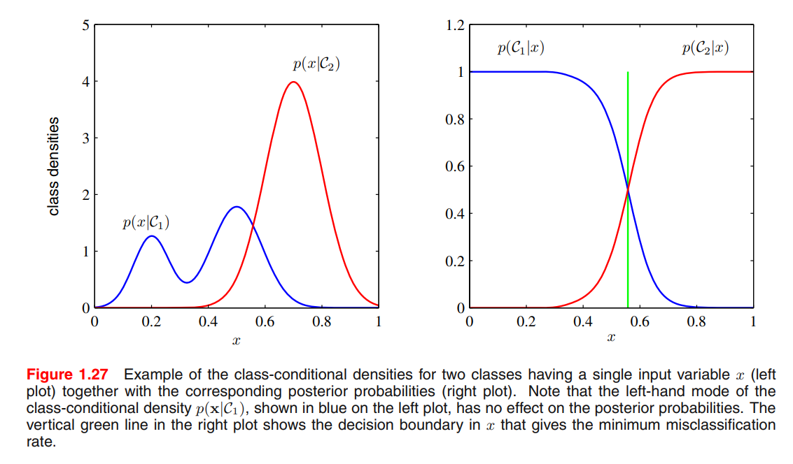
Decision Theory
Confusion Matrix
| Truth/Decision | Positive | Negative |
|---|---|---|
| Positive | TP | FN |
| Negative | FP | TN |
Receiver Operating Characteristic Curve
Minimizing the misclassification rate
$$
\begin{align*}
p(\text{correct})&=\sum\limits_{k=1}^Kp(\mathbf x\in\mathcal R_k,\mathcal C_k) = \sum\limits_{k=1}^K\int_{\mathcal R_k} p(\mathbf x,\mathcal C_k)\text d \mathbf x\
\end{align*}
$$
Minimizing the expected loss
$$
\mathbb E[L]=\sum\limits_k\sum\limits_j\int_{\mathcal R_j}L_{kj}p(\mathbf x,\mathcal C_k)\text d \mathbf x
$$
Each $\mathbf x$ can be assigned independently to one of the decision regions $\mathcal R_j$.
Goal is to choose $\mathcal R_j$ to minimize $\mathbb E[L]$, we should minimize $\sum\limits_{k} L_{kj}p(\mathbf x,\mathcal C_k)$ for each $\mathbf x$.
Common factor $p(\mathbf x)$ can be eliminated from $p(\mathbf x,\mathcal C_k)=p(\mathcal C_k\vert\mathbf x)p(\mathbf x)$.
Thus the decision rule that minimizes the expected loss is the one that assigns each new $\mathbf x$ to the class $j$ for which the quantity $\sum\limits_{k} L_{kj}p(\mathcal C_k\vert\mathbf x)$ is a minimum.
Reject Option
Introducing a threshold $\theta$ and rejecting those inputs $x$ for which the largest of the posterior probabilities $p(\mathcal C_k\vert \mathbf x)$ is less than or equal to $\theta$.
- $\theta=1$: all examples are rejected.
- $\theta<\frac 1 K$: ($K$ classes) no examples are rejected.
Inference and Decision
Generative model: Model the distribution of inputs as well as outputs. Because by sampling from them it is possible to generate synthetic data points in the input space.
Discriminative model: model the posterior probabilities directly.
Discriminant function: Learn a function that maps inputs x directly into decisions.
3 Ways to Solve Decision Problems
(a) By inference, determine $p(\mathbf x\vert \mathcal C_k)$ and $p(\mathcal C_k)$, then uses Bayes’ Theorem
$$
p(\mathcal C_k\vert\mathbf x)=\frac{p(\mathbf x\vert\mathcal C_k)p(\mathcal C_k)}{p(\mathbf x)}=\frac{p(\mathbf x\vert\mathcal C_k)p(\mathcal C_k)}{\sum\limits_{k}p(\mathbf x\vert\mathcal C_k)p(\mathcal C_k)}=\frac{p(\mathbf x,\mathcal C_k)}{\sum\limits_{k}p(\mathbf x,\mathcal C_k)}
$$
Equivalently, we can model the joint distribution $p(\mathbf x, \mathcal C_k)$ directly and then normalize to obtain the posterior probabilities. (generative model)(b) By inference, determine the posterior class probabilities $p(\mathcal C_k\vert\mathbf x)$ directly. (discriminative model)
(c) Find a function $f(x)$, called a discriminant function, which maps each input $\mathbf x$ directly onto a class label. Probabilities play no role.
Pros/Cons of the three approaches(extract from PRML)
Let us consider the relative merits of these three alternatives. Approach (a) is the most demanding because it involves finding the joint distribution over both
However, if we only wish to make classification decisions, then it can be wasteful of computational resources, and excessively demanding of data, to find the joint distribution
An even simpler approach is (c) in which we use the training data to find a discriminant function
With option (c), however, we no longer have access to the posterior probabilities
- Minimizing risk.
- Reject option.
- Compensating for class priors.
- Combining models.
Loss functions for regression
For each input $\bf x$, choose a specific estimation $y(\bf x)$ of the value $t$.
$$
\mathbb E[L]=\iint L(t,y(\mathbf x))p({\bf x},t)\text d {\bf x}\text dt
$$
Take squared loss $L(t,y({\bf x}))={y({\bf x})-t}^2$ for example
$$
\mathbb E[L]=\iint {y({\bf x})-t}^2p({\bf x},t)\text d {\bf x}\text dt
$$
Method 1. Calculus of Variations
Using a calculus of variations to give $y({\bf x})$ so as to minimize $\mathbb E[L]$:
$$
\frac{\partial \mathbb E[L]}{\partial y({\bf x})}=2\int {y({\bf x})-t}^2p({\bf x},t)\text d t =0
$$
Solving for $y({\bf x})$, and using the sum and product rules of probability, we obtain the regression function:
$$
y({\bf x})=\frac{\int tp({\bf x},t)\text d t}{p({\bf x})}=\int t p(t\vert \mathbf x)\text d t=\mathbb E_t[t\vert \mathbf x]
$$
which is the conditional average of $t$ conditioned on $\bf x$.
Method 2. Expanding the square term
$$
\begin{align*}
{y({\bf x})-t}^2&={y({\bf x})-\mathbb E_t[t\vert\mathbf x]+\mathbb E_t[t\vert\mathbf x]-t}^2\
&={y({\bf x})-\mathbb E_t[t\vert\mathbf x]}^2+2{y({\bf x})-\mathbb E_t[t\vert\mathbf x]}{\mathbb E_t[t\vert\mathbf x]-t}+{\mathbb E_t[t\vert\mathbf x]-t}^2
\end{align*}
$$
Substitute into the loss function and perform the integral on $t$:
$$
\mathbb E[L]=\int{y({\bf x})-\mathbb E_t[t\vert\mathbf x]}^2p(\mathbf x)\text d \mathbf x+\int{\mathbb E_t[t\vert\mathbf x]-t}^2p(\mathbf x)\text d\mathbf x
$$
When $y({\bf x})=\mathbb E_t[t\vert \mathbf x]$, loss function $\mathbb E[L]$ is minimized.
The second term represents the intrinsic variability of the target data and can be regarded as noise, or minimum value of the loss function.
3 Ways to Solve Regression Problems (in order of decreasing complexity)
- (a) Inference to determine the joint density $p({\bf x},t)$, then normalize to find the conditional density $p(t\vert \mathbf x)$, finally marginalize to find the conditional mean by the regression function.
- (b) Inference to determine the conditional density $p(t\vert \mathbf x)$, then marginalize to find the conditional mean by the regression function.
- (c) Find a regression function $y(\mathbf x)$ directly from the training data.
The relative merits of these three approaches follow the same lines as for classification problems.
Minkowski loss
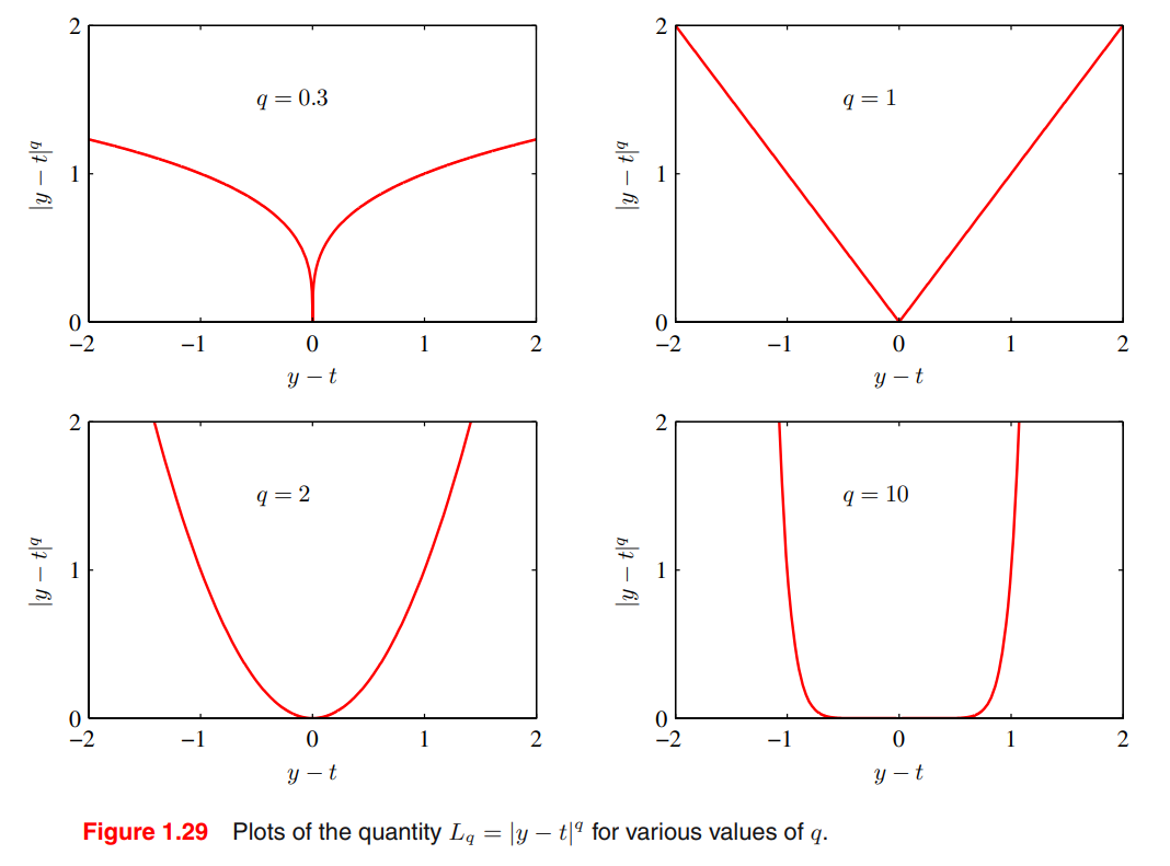
The minimum of $\mathbb E[L_q]$ is given by:
- $q\rightarrow 0$: conditional mode
- $q=1$: conditional median
- $q=2$: conditional mean
Information Theory
Entropy(statistical)
Discrete
Allocate $N$ identical objects in $M$ bins.
$$
W=\frac{N!}{\prod\limits_in_i!}
$$
$$
\text H=\frac 1 N \ln W\simeq -\lim\limits_{N\rightarrow\infty}\sum\limits_{i}(\frac{n_i}N)\ln(\frac{n_i}N)=-\sum\limits_{i}p_i\ln p_i
$$
Entropy maximized when $\forall i,\ p_i=\frac 1 M$.
Continuous
Put bins of width $\Delta$ along the real line.
$$
\lim\limits_{\Delta\rightarrow0}\left{-\sum\limits_{i}p(x_i)\Delta\ln p(x_i)\right}=-\int p(x)\ln p(x)\text d x
$$
For fixed $\sigma^2$, when $p(x)=\mathcal N(x\vert\mu,\sigma^2)$, differential entropy is maximized
$$
\text H[x]=\frac 1 2{1+\ln(2\pi\sigma^2)}
$$
Entropy
$$
\begin{align*}
\text H[x]&=-\sum\limits_x p(x)\ln p(x)\
\text H[x]&=-\int p(x)\ln p(x)\text d x
\end{align*}
$$
Conditional Entropy
$$
\text H[y\vert x]=-\iint p(\mathbf y,\mathbf x)\ln p(\mathbf y\vert\mathbf x)\text d\mathbf y\text d\mathbf x
$$
$$
\text H[\mathbf x,\mathbf y]=\text H[\mathbf y\vert\mathbf x]+\text H[\mathbf x]
$$
Relative Entropy (The Kullback-Leibler Divergence)
KL divergence describes a distance between model $p$ and model $q$.
$$
\begin{align*}
\text{KL}(p|q)&=\text{Cross Entropy C}(p|q)-\text {Entropy H}(p)\
&=-\int p(\mathbf x)\ln q(\mathbf x)\text d\mathbf x-\left(-\int p(\mathbf x)\ln p(\mathbf x)\text d\mathbf x\right)\
&=-\int p(\mathbf x)\ln \left{\frac{q(\mathbf x)}{p(\mathbf x)}\right}\text d\mathbf x
\end{align*}
$$
- It is not a symmetrical quantity: $\text{KL}(p|q)\not\equiv \text{KL}(q|p)$.
- $\text {KL}(p|q)\ge 0$, with equality IFF $p(\mathbf x)=q(\mathbf x)$.
Approximate distribution $p(\mathbf x)$ using distribution $q(\mathbf x\vert\boldsymbolθ)$ governed by a set of adjustable parameters $\boldsymbol\theta$. One way to determine $\boldsymbol\theta$ is to minimize the KL divergence between the two distributions.
$$
\text{KL}(p|q)\simeq \frac 1 N \sum\limits_{n=1}^N{\ln q(\mathbf x_n\vert\boldsymbol\theta)+\ln p(\mathbf x_n)}
$$
The 1st term is the negative log likelihood function for $\boldsymbol\theta$. The 2nd term is independent of $\boldsymbol\theta$. So minimizing this KL divergence is equivalent to maximizing the likelihood function.
Cross Entropy for Machine Learning
- Goal of ML: $p(\text{real data})\approx p(\text{model}\vert\theta)$
- We assume: $p(\text{training data})\approx p(\text{real data})$
- Operation of ML: $p(\text{training data})\approx p(\text{model}\vert\theta)$
Minimizing $\text{KL}(p(\text{training data})|p(\text{model}\vert\theta))$ is equivalent to minimizing $\text C(p(\text{training data})|p(\text{model}\vert\theta))$ as $\text H(p(\text{training data}))$ is fixed.
Example. Bernoulli model
$$
p(\text{model}\vert\theta)=\rho^t(1-\rho)^{1-t}
$$
$$
\text C=-\frac 1 N \sum\limits_nt_n\ln\rho+(1-t_n)\ln(1-\rho)
$$
where $t_n$ is the training data and $\rho$ is the model parameter.
Example. Gaussian model
$$
p(\text{model}\vert\theta)\propto e^{-\frac{(t-\mu)^2}{2}}
$$
$$
\text C\propto \frac 1 N \sum\limits_n(t_n-\mu)^2
$$
where $t_n$ is the training data and $\mu$ is the model parameter.
Mutual Information
Mutual information describes the degree of dependence between $\mathbf x$ and $\mathbf y$
$$
\begin{align*}
\text I[\mathbf x,\mathbf y]&\equiv\text{KL}(p(\mathbf x,\mathbf y)|p(\mathbf x)p(\mathbf y))\
&=-\iint p(\mathbf x,\mathbf y)\ln\left(\frac{p(\mathbf x)p(\mathbf y)}{p(\mathbf x,\mathbf y)}\right)\text d\mathbf x\text d\mathbf y
\end{align*}
$$
$$
\text I[\mathbf x,\mathbf y]=\text H[\mathbf x]-\text H[\mathbf x\vert\mathbf y]=\text H[\mathbf y]-\text H[\mathbf y\vert\mathbf x]
$$
Information Gain
Given $N$ balls and a balance, one of these balls is lighter.
$x$: one ball is lighter
$y$: weighing once
$\text H[x]$: uncertain of balls
$\text H[x\vert y]$: uncertain of balls after weighing once
$$
\begin{align*}
\text H[x\vert y_1,\cdots,y_t]-\text H[x\vert y_1,\cdots,y_{t+1}]&=\text H[y_{t+1}\vert y_1,\cdots,y_t]-H[y_{t+1}\vert y_1,\cdots,y_t,x]\
&=\text H[y_{t+1}\vert y_1,\cdots,y_t]\
&\le \text H[y_{t+1}]=\log_23
\end{align*}
$$
Sum the equation above with $t=0,1,\cdots,T$,
$$
\begin{matrix}
\log_2N = \text H[x]-\text H[x\vert y_1,\cdots,y_T]\le T\log_23\
T\ge \log_3N
\end{matrix}
$$
Chapter 3 - Distributions
Binary Distributions
Bernoulli Distribution
$$
\begin{align*}
\text{Bern}(x\vert \mu)&=\mu^x(1-\mu)^{1-x}\
\mathbb E[x]&=\mu\
\text{var}[x]&=\mu(1-\mu)
\end{align*}
$$
Given $\mathcal D={x_1,\cdots,x_N}$, $m$ heads, $N-m$ tails.
$$
\ln p(\mathcal D\vert\mu)=\sum\limits_{n=1}^N\ln p(x_n\vert\mu)=\sum\limits_{n=1}^N{x_n\ln\mu+(1-x_n\ln(1-\mu)}
$$
$$
\mu_\text{ML}=\frac 1 N\sum\limits_{n=1}^Nx_n=\frac m N
$$
Binomial Distribution
$$
\begin{align*}
\text{Bin}(m\vert N,\mu)&=\left(\begin{matrix}N\m\end{matrix}\right)\mu^m(1-\mu)^{N-m}\
\mathbb E[m]&=\sum\limits_{m=0}^Nm\text{Bin}(m\vert N,\mu)=N\mu\
\text{var}[m]&=\sum\limits_{m=0}^N(m-\mathbb E[m])^2\text{Bin}(m\vert N,\mu)=N\mu(1-\mu)
\end{align*}
$$
Beta Distribution
$$
\begin{align*}
\Gamma(x)&\equiv\int_0^\infty u^{x-1}e^{-u}du\
\text{Beta}(\mu\vert a,b)&=\frac{\Gamma(a+b)}{\Gamma(a)\Gamma(b)}\mu^{a-1}(1-\mu)^{b-1}\
\mathbb E[\mu]&=\frac a {a+b}\
\text{var}[\mu]&=\frac{ab}{(a+b)^2(a+b+1)}
\end{align*}
$$
The Beta distribution provides the conjugate prior for the Bernoulli distribution.
Given $\mathcal D={x_1,\cdots,x_N}$, $m$ heads, $N-m$ tails.
$$
\begin{matrix}
p(\mu\vert a_0,b_0,\mathcal D)\propto p(\mathcal D\vert\mu)p(\mu\vert a_0,b_0)\propto \text{Beta}(\mu\vert a_N,b_N)\
a_N=a_0+m\quad\quad b_N=b_0+(N-m)
\end{matrix}
$$
As the size of the dataset $N$ increases,
$$
\begin{align*}
a_N &\rightarrow m\
b_N &\rightarrow N-m\
\mathbb E[\mu]&\rightarrow \mu_\text{ML}\
\text{var}[\mu]&\rightarrow 0
\end{align*}
$$
Multinomial Distributions
1-of-K coding scheme
1-of-K coding scheme: $\mathbf x=(0,0,1,0,0,0)^\text T,\ \sum\limits_{k=1}^Kx_k=1$.
$$
p(\text x\vert\boldsymbol\mu)=\prod\limits_{k=1}^K\mu_k^{x_k}
$$
where $\boldsymbol\mu=(\mu_1,\cdots,\mu_K)^\text T$, $\sum\limits_k\mu_k=1$.
$$
\mathbb E[\mathbf x\vert\boldsymbol \mu]=\sum\limits_{\mathbf x}p(\mathbf x\vert\boldsymbol\mu)\mathbf x=(\mu_1,\cdots,\mu_K)^\text T=\boldsymbol \mu
$$
Given $\mathcal D={\bf x_1,\cdots,x_N}$, the likelihood
$$
p(\mathcal D\vert\mu)=\prod\limits_{n=1}^N\prod\limits_{k=1}^K\mu_k^{x_{nk}}=\prod_{k=1}^K\mu_k^{\left(\sum\limits_{n=1}^Nx_{nk}\right)}=\prod_{k=1}^K\mu_k^{m_k}
$$
where $ m_k=\sum\limits_{n=1}^Nx_{nk}$ denotes the number of observations of $x_k = 1$.
Using Lagrange method, we obtain
$$
\mu^\text{ML}_k=\frac {m_k} N
$$
Multinomial Distribution
$$
\begin{align*}
\text{Mult}(m_1,\cdots,m_K\vert\boldsymbol\mu,N)&=\left(\begin{matrix}N\m_1\cdots m_K\end{matrix}\right)\prod\limits_{k=1}^K\mu_k^{m_k}\
\mathbb E[m_k]&=N\mu_k\
\text{var}[m_k]&=N\mu_k(1-\mu_k)\
\text{cov}[m_jm_k]&=-N\mu_j\mu_k
\end{align*}
$$
Dirichlet Distribution
Conjugate prior for the multinomial distribution.
$$
\begin{matrix}
\text{Dir}(\boldsymbol\mu\vert\boldsymbol\alpha)=\frac{\Gamma(\alpha_0)}{\Gamma(\alpha_1)\cdots\Gamma(\alpha_K)}\prod\limits_{k=1}^K\mu_k^{\alpha_k-1}\
\alpha_0=\sum\limits_{k=1}^K\alpha_k
\end{matrix}
$$
Given $\mathcal D={m_1,\cdots,m_K}$, the likelihood
$$
\begin{matrix}
p(\boldsymbol\mu\vert\mathcal D,\boldsymbol\alpha)\propto p(\mathcal D\vert\boldsymbol\mu)p(\boldsymbol\mu\vert\boldsymbol\alpha)\propto\prod\limits_{k=1}^K\mu_k^{\alpha_k+m_k-1}\
p(\boldsymbol\mu\vert\mathcal D,\boldsymbol\alpha)=\text{Dir}(\boldsymbol\mu\vert\boldsymbol\alpha+\bf m)
\end{matrix}
$$
where $\mathbf m=(m_1,\cdots,m_K)^\text T$.
We can interpret the parameters $\alpha_k$ of the Dirichlet prior as an effective number of observations of $x_k = 1$.
Gaussian Distributions
The Gaussian Distribution
$$
\mathcal N(x|\mu,\sigma^2)=\frac 1 {(2\pi\sigma^2)^{1/2}}\exp\left{-\frac 1 {2\sigma^2}(x-\mu)^2\right}
$$The Multivariate Gaussian
$$
\mathcal N(\mathbf x|\mathbf\mu,\mathbf\Sigma)=\frac 1 {(2\pi)^{D/2}}\frac 1 {|\mathbf\Sigma|^{1/2}}\exp\left{-\frac 1 2(\mathbf x-\mathbf\mu)^\text T\mathbf\Sigma^{-1}(\mathbf x - \mathbf \mu)\right}
$$
Central Limit Theorem
The distribution of the sum of $N$ i.i.d. random variables becomes increasingly Gaussian as $N$ grows.
Moments of the Multivariate Gaussian
$$
\begin{align*}
\mathbb E[\mathbf x]&=\boldsymbol\mu\
\mathbb E[\mathbf x\mathbf x^\text T]&=\boldsymbol\mu\boldsymbol\mu^\text T+\boldsymbol\Sigma\
\text{cov}[\mathbf x]&=\boldsymbol\Sigma\
\text{cov}[A\mathbf x]&=A\boldsymbol\Sigma A^\text T
\end{align*}
$$
Properties of Gaussians
- Linear transformation
$$
\begin{align*}
X&\sim\mathcal N(\mu,\sigma^2)\
Y&=aX+b\
Y&\sim\mathcal N(a\mu+b,a^2\sigma^2)
\end{align*}
$$
Product of Gaussian r.v.
$$
\begin{align*}X_1&\sim\mathcal N(\mu_1,\sigma_1^2)\X_2&\sim\mathcal N(\mu_2,\sigma_2^2)\
p(Y)&=p(X_1)p(X_2)\
Y&\sim\mathcal N(\frac{\sigma^2_2}{\sigma_1^2+\sigma_2^2}\mu_1+\frac{\sigma^2_1}{\sigma_1^2+\sigma_2^2}\mu_2,\frac 1 {\sigma_1^{-2}+\sigma_2^{-2}})
\end{align*}
$$$$
\left{\begin{align*}\sigma^{-2}&=\sigma_1^{-2}+\sigma_2^{-2}\\sigma^{-2}\mu&=\sigma_1^{-2}\mu_1+\sigma_2^{-2}\mu_2\end{align*}\right .
$$For multivariate Gaussians, use $\Sigma$ to replace $\sigma^2$.
Bayes’ Theorem for Gaussian Variables(Slides)
Given $y=Ax+v$, $p(x)=\mathcal N(x\vert\mu,\Sigma)$, $p(v)=\mathcal N(v\vert,0,Q)$.
Hence we have
$$
\begin{align*}
p(y)&=\mathcal N(y\vert A\mu,A\Sigma A^\text T+Q)\
p(y\vert x)&=\mathcal N(y\vert Ax,Q)
\end{align*}
$$
Therefore
$$
\begin{align*}
p(x\vert y)&\propto p(y\vert x)p(x)=\mathcal N(y\vert Ax,Q)\mathcal N(x\vert \mu,\Sigma)\
p(x\vert y) &= \mathcal N(x\vert Hy,L)\
\end{align*}
$$
where
$$
\left{ \begin{align*}
L^{-1}&=A^TQ^{-1}A + \Sigma^{-1}\
Hy &= L{A^TQ^{-1}y+\Sigma^{-1}\mu}
\end{align*}\right.
$$
Conditional Gaussian distributions
If two sets of variables are jointly Gaussian, then the conditional distribution of one set conditioned on the other is again Gaussian.
Given a $D$-dimensional vector $\mathbf x$ with Gaussian distribution $\mathcal N(\mathbf x\vert\boldsymbol\mu,\boldsymbol\Sigma)$, partitioned into two disjoint subsets $\mathbf x_a$ and $\mathbf x_b$.
$$
\mathbf x=\left(\begin{matrix}\mathbf x_a\\mathbf x_b\end{matrix}\right)\quad\boldsymbol\mu=\left(\begin{matrix}\boldsymbol \mu_a\\boldsymbol \mu_b\end{matrix}\right)\quad\boldsymbol\Sigma=\begin{pmatrix}\boldsymbol\Sigma_{aa}&\boldsymbol\Sigma_{ab}\\boldsymbol\Sigma_{ba}&\boldsymbol\Sigma_{bb}\end{pmatrix}
$$
For conditional distribution $p(\mathbf x_a\vert\mathbf x_b)$,
$$
\begin{align*}
p(\mathbf x_a\vert\mathbf x_b)&=\mathcal N(x_a\vert\boldsymbol\mu_{a\vert b},\boldsymbol\Sigma_{a\vert b})\
\boldsymbol\mu_{a\vert b}&=\boldsymbol\mu_a+\boldsymbol\Sigma_{ab}\boldsymbol\Sigma_{bb}^{-1}(\mathbf x_b-\boldsymbol\mu_b)\
\boldsymbol\Sigma_{a\vert b}&=\boldsymbol\Sigma_{aa}-\boldsymbol\Sigma_{ab}\boldsymbol\Sigma_{bb}^{-1}\boldsymbol\Sigma_{ba}
\end{align*}
$$
And marginal distribution $p(\mathbf x_a)=\mathcal N(\mathbf x_a\vert\boldsymbol\mu_a,\boldsymbol\Sigma_{aa})$.
Bayes’ Theorem for Gaussian Variables(Textbook)
Given
$$
\begin{align*}
p(\mathbf x)&=\mathcal N(\mathbf x\vert\boldsymbol\mu,\boldsymbol\Lambda^{-1})\
p(\mathbf y\vert \mathbf x)&=\mathcal N(\bf y\vert Ax+b, L^{-1})
\end{align*}
$$
Obtain
$$
\begin{align*}
p(\mathbf y)&=\mathcal N(\bf y\vert A\mu+b,L^{-1}+A\Lambda^{-1}A^\text T)\
p(\mathbf x\vert\mathbf y)&=\mathcal N(\bf x\vert\boldsymbol \Sigma{A^\text TL(y-b)+\Lambda\boldsymbol\mu},\Sigma)
\end{align*}
$$
where
$$
\boldsymbol\Sigma=(\bf\Lambda+A^\text{T}LA)^{-1}.
$$
Maximum Likelihood for the Gaussian
Sufficient statistics: $\sum\limits_{n=1}^N\mathbf x_n$ and $\sum\limits_{n=1}^N\mathbf x_n\mathbf x_n^\text T$
Solve the maximum likelihood
$$
\boldsymbol\mu_\text{ML}=\frac 1 N\sum\limits_{n=1}^N\mathbf x_n\quad \boldsymbol\Sigma_\text{ML}=\frac 1 N\sum\limits_{n=1}^N(\mathbf x_n-\boldsymbol\mu_\text{ML})(\mathbf x_n-\boldsymbol\mu_\text{ML})^\text T.
$$
Under the true distribution
$$
\mathbb E[\boldsymbol \mu_\text{ML}]=\boldsymbol\mu\quad\mathbb E[\boldsymbol \Sigma_\text{ML}]=\frac{N-1}N\boldsymbol\Sigma.
$$
Hence define
$$
\widetilde{\boldsymbol\Sigma}=\frac 1 {N-1}\sum\limits_{n=1}^N(\mathbf x_n-\boldsymbol\mu_\text{ML})(\mathbf x_n-\boldsymbol\mu_\text{ML})^\text T.
$$
Sequential estimation
Bayesian Inference for the Gaussian
Student’s t-distribution
Periodic variables
Mixtures of Gaussians
$$
p(\mathbf x)=\sum\limits_{k=1}^K\pi_k\mathcal N(\mathbf x\vert\boldsymbol\mu_k,\boldsymbol\Sigma_k)
$$
$\pi_k$: mixing coefficients
$\sum\limits_{k=1}^K\pi_k=1,0\le\pi_k\le 1$
$N(\mathbf x\vert\boldsymbol\mu_k,\boldsymbol\Sigma_k)$: component
Log likelihood of mixtures
$$
\ln p(\mathbf X\vert\boldsymbol \pi,\boldsymbol\mu,\boldsymbol\Sigma)=\sum\limits_{n=1}^N\ln\left{\sum\limits_{k=1}^K\pi_k\mathcal N(\mathbf x\vert\boldsymbol\mu_k,\boldsymbol\Sigma_k)\right}
$$
The maximum likelihood solution for the parameters no longer has a closed-form analytical solution.
Alternatives: iterative numerical optimization, expectation maximization.
Exponential Families
The exponential family of distributions over $\mathbf x$, given parameters $\boldsymbol \eta$
$$
p(\mathbf x\vert\boldsymbol\eta)=h(\mathbf x)g(\boldsymbol\eta)\exp{\boldsymbol\eta^\text T\mathbf u(\mathbf x)}
$$
- $\bf x$: scalar or vector, discrete or continuous.
- $\boldsymbol\eta$: natural parameters
- $g(\boldsymbol\eta)$: normalization coefficient satisfying ↓
$$
g(\boldsymbol\eta)\int h(\mathbf x)\exp\left{\boldsymbol\eta^\text T \mathbf u(\mathbf x)\right}\text d\mathbf x=1
$$
The Bernoulli Distribution:
$$
p(x\vert \mu)=(1-\mu)\exp\left{\ln(\frac{\mu}{1-\mu})x\right}
$$
So
$$
\begin{align*}
\eta = \ln(\frac \mu{1-\mu}), \mu=&\sigma(\eta)=\frac 1{1+\exp(-\eta)}\
&\uparrow\text{Logistic Sigmoid}
\end{align*}
$$
The Multinomial Distribution:
$$
p(\mathbf x\vert\boldsymbol \mu)=\exp\left{\sum\limits_{k=1}^Mx_k\ln\mu_k\right}
$$
Let $\mu_M=1-\sum\limits_{k=1}^{M-1}\mu_k$,
$$
\begin{align*}
\eta_k=\ln\left(\frac {\mu_k} {1-\sum_{j=1}^{M-1}\mu_j}\right), \mu_k = &\frac{\exp(\eta_k)}{1+\sum_{j=1}^{M-1}\exp(\eta_j)}\
&\uparrow\text{Softmax}
\end{align*}
$$
The Gaussian Distribution:
$$
p(x\vert\mu,\sigma^2)=\frac 1 {\sqrt{2\pi\sigma^2}}\exp\left{-\frac 1 {2\sigma^2}(x-\mu)^2\right}=h(x)g(\boldsymbol\eta)\exp\left{\boldsymbol\eta^\text T\mathbf u(x)\right}
$$
where
$$
\begin{align*}
\boldsymbol\eta &= \left(\begin{matrix}\frac{\mu}{\sigma^2}\\frac {-1} {2\sigma^2}\end{matrix}\right) &h(x) &= \frac{1}{\sqrt{2\pi}}\
\mathbf u(x) &= \left(\begin{matrix}x\x^2\end{matrix}\right) &g(\boldsymbol\eta) &= \sqrt{-2\eta_2}\exp\left(\frac{\eta_1^2}{4\eta_2}\right)
\end{align*}
$$
Maximum likelihood and sufficient statistics
Likelihood function
$$
p(\mathbf{X} \vert \boldsymbol{\eta})=\left(\prod_{n=1}^{N} h\left(\mathbf{x}{n}\right)\right) g(\boldsymbol{\eta})^{N} \exp \left{\boldsymbol{\eta}^{T} \sum{n=1}^{N} \mathbf{u}\left(\mathbf{x}{n}\right)\right}
$$
Condition of maximum likelihood estimator $\boldsymbol\eta\text{ML}$
$$
\begin{align*}
-\nabla\ln g(\boldsymbol \eta_\text{ML})=\frac 1 N& \sum\limits_{n=1}^N\mathbf u(\mathbf x_n)\
&\uparrow\text{Sufficient statistic}
\end{align*}
$$
The solution for the ML estimator only depends on $\sum\limits_{n=1}^N\mathbf u(\mathbf x_n)$, which is called the sufficient statistic of the distribution.
For example,
Bernoulli distribution $\mathbf u(x) = x$, so we only keep the sum of the data points; Gaussian distribution $\mathbf u(x) = \left(\begin{matrix}x\x^2\end{matrix}\right)$, we need to keep both the sum of data points and the sum of the square.
Conjugate Priors
Seek a prior that is conjugate to the likelihood function: the posterior distribution has the same functional form as the prior.
For any member of the exponential family, there exists a conjugate prior
$$
\text{prior} = p(\boldsymbol\eta\vert\chi,\nu) = f(\chi,\nu)g(\boldsymbol\eta)^\nu\exp\left{\nu\boldsymbol\eta^\text T\chi\right}
$$
where
- $f(\chi,\nu)$ is a normalization coefficient
- $g(\boldsymbol\eta)$ is the normalization coefficient of the exponential family.
Recall that
$$
\text{Likelihood} =p(\mathbf{X} \vert \boldsymbol{\eta})=\left(\prod_{n=1}^{N} h\left(\mathbf{x}{n}\right)\right) g(\boldsymbol{\eta})^{N} \exp \left{\boldsymbol{\eta}^{T} \sum{n=1}^{N} \mathbf{u}\left(\mathbf{x}{n}\right)\right}
$$
Multiply the prior and the likelihood, the posterior is
$$
\text{Posterior} \propto g(\boldsymbol\eta)^{\nu+N}\exp\left{\boldsymbol\eta^\text T \left(\sum\limits{n=1}^N\mathbf u(\mathbf x_n)+\nu\chi\right)\right}
$$
which is in the same functional form as the prior.
- $\nu$: effective number of pseudo-observations in the prior
- $\chi$: value of the sufficient statistic for the pseudo-observations
Non-informative Priors
Used when little is known about the prior distribution.
Have as little influence on the posterior distribution as possible.
Cons of choose constant as the prior
- If the domain of the parameter $\lambda$ is unbounded, the integral over $\lambda$ diverges, hence the prior cannot be normalized and is improper.
- By changing the variable(e.g., $\lambda=\eta^2$), the density over the new variable may not be constant.
Example: $\text{Gam}(\lambda\vert a_0,b_0)$ where $a_0=b_0=0$.
Non-parametric Methods
Limitation of parametric methods:
The chosen density might be a poor model of the distribution that generates the data. Multimodal data can never be captured by a unimodal Gaussian.
Histogram Methods
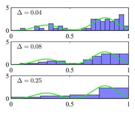 $$
p_i = \frac{n_i}{N\Delta_i}
$$
where $\Delta$ acts as a smoothing parameter.
$$
p_i = \frac{n_i}{N\Delta_i}
$$
where $\Delta$ acts as a smoothing parameter.
Cons: Curse of Dimensionality
K-Nearest-Neighbors
Chapter 4 - Linear Models for Regression
Chapter 5 - Linear Models for Classification
Three Approaches to Classification
- Use discriminant functions directly
- Infer the posterior probabilities with generative models
- Directly construct posterior conditional class probabilities
Discriminant Functions
Discriminant Functions for $N$ classes
- use $N$ two-way discriminant functions
- use $\frac{N(N-1)}{2}$ two-way discriminant functions
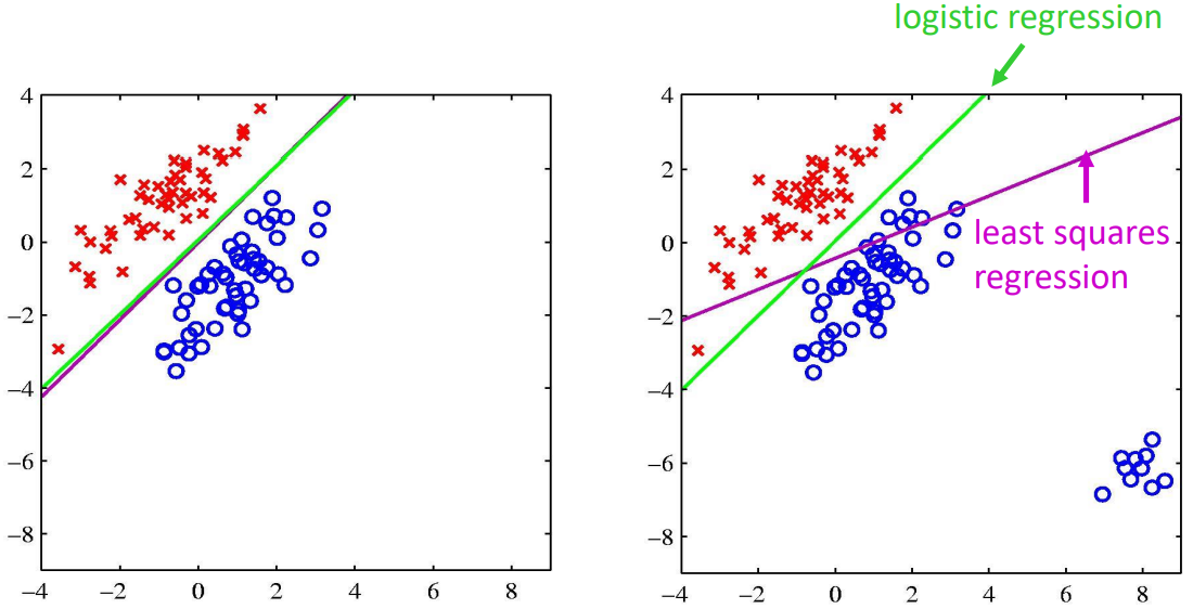
Least Square Classification
- Reduce classification to least squares regression.
- Treat each class as a separate problem, pick the max.
Least square regression is sensitive to outliers, use logistic regression to solve this problem:
Fisher’s Linear Discriminants(LDA)
See the course material for Lab06: LDA
Perceptron
$$
y(\mathbf x)=f(\mathbf w^\text T\phi(\mathbf x))\quad f(a) = \left{\begin{matrix}+1,a\ge0 \ -1, a<0\end{matrix}\right.
$$
Training
Criterion:
$$
E_P(\mathbf w)=-\sum\limits_{n\in\mathcal M}\mathbf w^\text T\phi_nt_n
$$
where $t_n\in{1,-1}$ is the label.
$$
\mathbf w^{(\tau+1)}=\mathbf w^\tau-\eta\nabla E_P(\mathbf w)=\mathbf w^\tau + \eta\phi_nt_n
$$
where $\eta$ is the learning rate.
$$
-\mathbf (w^{(\tau+1)})^\text T\phi_nt_n<-(w^{\tau})^\text T\phi_nt_n
$$
indicating the convergence of perceptron training.
Simplified Training
$$
\mathbf w^\text{new}=\mathbf w^\text{old}-0.5(y_n-t_n)x_n
$$
- guaranteed to find a set of weights that gets the right answer on the whole training set if any such a set exists.
- no need to choose a learning rate.
Probabilistic Generative Models
$$
p(C_1\vert\mathbf x)=\frac{p(C_1)p(\mathbf x\vert C_1)}{p(\mathbf x)}=\frac{1}{1+e^{-z}}=\sigma(z)
$$
where $z$ is called the logit
$$
z=\ln\frac{p(C_1)p(x\vert C_1)}{\sum\limits_{i\neq 1}p(C_i)p(x\vert C_i)}=\ln \frac{p(C_1\vert \mathbf x)}{1-p(C_1\vert \mathbf x)}
$$
K-Case Classification
$$
p(C_k\vert\mathbf x)=\frac{p(C_k)p(\mathbf x\vert C_k)}{\sum\limits_{i}p(C_i)p(x\vert C_i)}
$$
Generative: ML Gaussian Mixtures
$$
\begin{array}{l}
p(x, C_{1})=p(C_{1}) p(x \vert C_{1})=\pi \mathcal N(x \vert \mu_{1}, \Sigma) \
p(x, C_{2})=p(C_{2}) p(x \vert C_{2})=(1-\pi) \mathcal N(x \vert \mu_{2}, \Sigma)
\end{array}
$$
Likelihood $p\left(\boldsymbol{t}, \boldsymbol{X} \vert \pi, \mu_{1}, \mu_{2}, \Sigma\right)=\prod_{n=1}^{N}\left[\pi N\left(x_{n} \vert \mu_{1}, \Sigma\right)\right]^{t_{n}}\left[(1-\pi) N\left(x_{n} \vert \mu_{2}, \Sigma\right)\right]^{1-t_{n}}$
$$
\begin{align*}
\pi_{M L}&=\frac{1}{N} \sum_{n=1}^{N} t_{n}=\frac{N_{1}}{N}=\frac{N_{1}}{N_{1}+N_{2}} \
\mu_{1 \mathrm{ML}}&=\frac{1}{N_{1}} \sum_{n=1}^{N} t_{n} x_{n} \ \mu_{2 \mathrm{ML}}&=\frac{1}{N_{2}} \sum_{n=1}^{N}\left(1-t_{n}\right) x_{n} \
\Sigma&=\pi \Sigma_{1}+(1-\pi) \Sigma_{2} \ \Sigma_{i \mathrm{ML}}&=\frac{1}{N_{i}} \sum_{x_{n} \in C_{i}}\left(x_{n}-\mu_{i}\right)\left(x_{n}-\mu_{i}\right)^{T} \quad \mathrm{i}=1,2
\end{align*}
$$
Generative: MAP Gaussian Mixtures
$$
\pi_0=\frac{N_{10}}{N_{10}+N_{20}}, x\in\mathcal C_i\sim(x\vert\mu_{i0},\Sigma_{i0})
$$
$$
\pi_\text{MAP} = \frac{N_1+N_{10}}{N+N_0}=\frac{N_1+N_{10}}{N_1+N_2+N_{10}+N_{20}}
$$
$$
\left{\begin{align*}\Sigma_{i\text{MAP}}^{-1}&=\Sigma_{i\text{ML}}^{-1}+\Sigma_{i0}^{-1}\\Sigma_{i\text{MAP}}^{-1}\mu_{i\text{MAP}}&=\Sigma_{i\text{ML}}^{-1}\mu_{i\text{ML}}+\Sigma_{i0}^{-1}\mu_{i0}\end{align*}\right.
$$
Probabilistic Discriminative Models
Bayesian Information Criterion
Chapter 6 - Neural Networks

Chapter 7 - Sparse Kernel Machines
Support Vector Machines
Model: $\quad y(\mathbf x) = \mathbf w^\text T \phi(\mathbf x) + b$
Distance of a point to the decision surface
$$
\frac{t_ny(\mathbf x_n)}{\vert\vert \mathbf w \vert\vert} = \frac{t_n(\mathbf w^\text T \phi(\mathbf x) + b)}{\vert\vert \mathbf w \vert\vert}
$$
Rescaling $\mathbf w$ and $b$, the point closest to the surface(active constraint) satisfies:
$$
\quad t_n(\mathbf w^\text T \phi(\mathbf x) + b)=1
$$
Then the classification problem becomes:
$$
\mathop{\arg\min}\limits_{\mathbf w, b} \frac 1 2 \vert\vert\mathbf w\vert\vert^2 \text{ subject to } t_n(\mathbf w^\text T \phi(\mathbf x) + b)\ge 1,\ n=1,\dots,N
$$
Hard Margin Classifier
The classification problem:
$$
\mathop{\arg\min}\limits_{\mathbf w, b} \sum\limits_{n=1}^N E_\infty (y(\mathbf x_n)t_n-1)+\lambda\vert\vert\mathbf w\vert\vert^2,\quad\lambda>0
$$
where
$$
E_\infty(z) = \left{\begin{matrix}0, &z\ge 0 \ \infty, &z<0\end{matrix}\right.
$$
Soft Margin Classifier
Introduce slack variables $\xi_n\ge 0, n=1,\dots,N$ (sometimes $\xi_n<0$ is allowed)
The classification problem:
$$
\begin{align*}
&\mathop{\arg\min}\limits_{\mathbf w, b}\ \ C\sum\limits_{n=1}^N \xi_n+\frac 1 2 \vert\vert\mathbf w\vert\vert^2 \&\text{ subject to } t_n(\mathbf w^\text T \phi(\mathbf x) + b)\ge 1,\ n=1,\dots,N
\end{align*}
$$
where $C>0$ is the trade-off between minimizing training errors and controlling model complexity.
SVMs and Logistic Regression
Multiclass SVMs
- One vs. Rest: $K$ separate SVMs
- Can lead to inconsistent results
- Imbalanced training sets
- One vs. One: $\frac{K(K-1)}{2}$ SVMs
- dead zone
SVMs for Regression
过的很快,只用了一分半
※Relevance Vector Machines
Given an input vector $\mathbf x$, the conditional distribution for a real-valued target variable $t$:
$$
p(t\vert\mathbf x,\mathbf w,\beta) = \mathcal N(t\vert y(\mathbf x),\beta^{-1})
$$
where $\beta=\sigma^{-2}$ is the noise precision.
The mean is given by a linear model, which can be written in an SVM-like form:
$$
y(\mathbf x) = \sum\limits_{n=1}^N w_nk(\mathbf x,\mathbf x_n)+b
$$
where $k(\mathbf x,\mathbf x_n)=\phi(\mathbf x)^\text T \phi(\mathbf x_n)$ is the kernel, and $b$ is 616.a bias parameter.
Chapter 8 - Mixture Models and EM Learning
Chapter 9 - Sequential Data
Conditional data: independent of the previous states
Sequential data: dependent of the previous states
Markov models
first-order:
$$
\begin{align*}
p(\mathbf x_1,\dots,\mathbf x_N) &= p(\mathbf x_1) \prod\limits_{n=2}^N p(\mathbf x_n\vert\mathbf x_{n-1})\
p(\mathbf x_n\vert\mathbf x_1,\dots,\mathbf x_{n-1}) &= p(\mathbf x_n\vert\mathbf x_{n-1})
\end{align*}
$$second-order:
$$
p(\mathbf x_1,\dots,\mathbf x_N) = p(\mathbf x_1)p(\mathbf x_2\vert\mathbf x_1) \prod\limits_{n=3}^N p(\mathbf x_n\vert\mathbf x_{n-1},\mathbf x_{n-2})
$$
Hidden Markov Models
For each observation $\mathbf x_n$, introduce latent variable $\mathbf z_n$, such that $\mathbf z_{n+1}\perp!!!!\perp \mathbf z_{n-1} \vert \mathbf z_n$
$$
p(\mathbf x_1,\dots,\mathbf x_N,\mathbf z_1,\dots,\mathbf z_N) = p(\mathbf z_1)[\prod\limits_{n=2}^N]p(\mathbf z_n\vert\mathbf z_{n-1})\prod\limits_{n=1}^N p(\mathbf x_n\vert\mathbf z_n)
$$
Use 1-of-K encoding, the latent variable is K-dimensional binary vector. The transition probability matrix $A_{j,k}\equiv p(z_{n,k}=1\mid z_{n-1,j}=1)$. This matrix satisfies $\sum\limits_{k} A_{jk}=1$ therefore has $K(K-1)$ independent parameters.
Chapter 10 - Markov Decision Process
Markov Decision Process
Given states $x$, actions $u$, transition probabilities $p(x’\mid u,x)$, reward function $r(x,u)$.
Expected cumulative reward:
$$
R_T^\pi(x_t) = \mathbb E[\sum\limits_{\tau=1}^T \gamma ^\tau r_{t+\tau}\mid u_{t+\tau} = \pi(z_{1:t+\tau-1},u_{1:t+\tau-1})]
$$
- $T=1$: greedy
- $T>1$: finite horizon
- $T=\infty$: infinite horizon
Goal: optimal policy
$$
\pi^\star = \mathop{\arg\max}\limits_{\pi}\ R_T^\pi(x_t)
$$
T-Step Policy and Value Function
$$
\begin{align}
V_T(x) &= \gamma \max\limits_u[r(x,u)+\int V_{T-1}(x’)p(x’\mid u,x)\text d x’]\
\pi_T(x) &= \mathop{\arg\max}\limits_u [r(x,u)+\int V_{T-1}(x’)p(x’\mid u,x)\text d x’]
\end{align}
$$
Value Iteration and Policy Iteration

